McCarty Group Wiki

Umbrella Sampling

Umbrella sampling and weighted histogram analysis (WHAM) in GROMACS with PLUMED2

About this tutorial

In this tutorial we will use GROMACS patched with PLUMED2 to compute the potential of mean force (PMF) using umbrella sampling and weighted histogram analysis (WHAM). As an example system we will compute the PMF between two methane molecules in water. This tutorial was created using GROMACS-2019.4 and PLUMED2.7.0. The necessary files to run this tutorial can be found here.

Summary of theory

In umbrella sampling, multiple simulations are performed in which the potential energy of the system is biased with a harmonic potential of the form

where \(\xi\) is the reaction coordinate. Different umbrella windows are employed with the potential centered on successive values of \(\xi_i\). The region sampled in the presence of the biasing potential is called a window. Configurations within each biased simulation \(i\) are sampled according to the distribution

where R are the atomic coordinates, \(k_B\) is the Boltzmann constant, \(T\) is the temperature, and \(P(R)\) is the Boltzmann distribution

The sampling in each umbrella window is confined to a narrow region around \(\xi_i\) due to the harmonic constraint, forcing the system to explore only a predefined region of the reaction coordinate. By combining simulations performed with different values of \(\xi_i\), we can compute the continuous potential of mean force along the reaction coordinate.

The weighted histogram analysis method (WHAM) provides a scheme for obtaining the optimal estimate of the unbiased probability distribution from the biased probability distributions due to the biasing potentials. The WHAM equations are

where \(N_w\) is the number of sampling windows, and \(n_i\) is the number of configuratoins for a biased simulation. Equations \(\ref{EQ:WHAM1}\) and \(\ref{EQ:WHAM2}\) must be solved self-consistently since the \(F_j\)s are unknown.

Umbrella Sampling in GROMACS without PLUMED2

In this section we will demonstrate the GROMACS implementation of WHAM. This part of the tutorial follows closely that from the Svedružić lab. First we need to set up our system. You will need a pdb file for a single methane molecule, here called methane.pdb. We will use the OPLS force field parameters for methane and the TIP4PEW water model. First you need to copy the methane.rtp file to the oplsaa.ff directory (usually in /usr/local/gromacs/share/gromacs/top/). Now we can use pdb2gmx to create a GROMACS .gro and .top file:

gmx pdb2gmx -f methane.pdb

When prompted select the OPLS-AA/L all-atom force field and the TIP4PEW TIP 4-point with Ewald water model. Running the pdb2gmx command will create a topology file topol.top and a conf.gro structure file.

Now we will insert two methane molecules randomly in a 0.5 nm box as follows:

gmx insert-molecules -ci methane.pdb -o box.gro -nmol 2 -box 0.5 0.5 0.5

This ensures the inserted molecules are not too far apart in our initial configuration. Now we will make the box bigger to the desired box size (for this tutorial we need a box size of at least 3.2 nm):

gmx editconf -f box.gro -o newbox.gro -c -box 3.2 3.2 3.2

Open the topol.top file in a text editor of your choice and update the last line to the correct number of methanes from 1 to 2.

[ molecules ]
; Compound       #mols
Other              2

Then add water to the box:

gmx solvate -cs tip4p -cp newbox.gro -o conf.gro -p topol.top -maxsol 1000

Finally, to perform umbrella sampling in GROMACS we will need to create an index file using make_ndx to make two groups that will be used in specifying the restraining potential. Here we will create a group containing just one carbon from each of the two methanes and name them CA and CB respectively.

gmx make_ndx -f conf.gro

splitres 2

6 & a C
7 & a C

name 8 CA
name 9 CB
q

We are now ready to perform the umbrella sampling simulations. We will perform 27 simulation windows with a harmonic restraint center at 0.05 nm to 1.3 nm. The are different ways in which we could generate our initial configurations for each window. In this tutorial, we will perform a two-stage energy minimization of each window. In the first stage we minimize the energy of the system with a maximum of 1,000 steps. We have included the flag define = -DFLEXIBLE, which signals to use flexible water, since by default all water models are rigid using an algorithm called SETTLE. In the second minimization we remove the define = -DFLEXIBLE and increasing the maximum number of steps to 50,000 to get the molecules in a good starting position. Then, we will equilibrate each window for 100 ps in the NVT ensemble followed by a 1 ns equilibration in the NPT ensemble.

Since the umbrella potential is applied during the equilibrations, the methanes should get to the correct distances during the equilibration stage due to the bias potentials. Lastly, we will run a 5 ns production run.

All the .mdp files are provided in the directory mdp-pull. The important thing to notice in the .mdp files is the introduction of the COM pulling feature of GROMACS. This is set with the lines

pull                  = yes         ; Use the pull code
pull-ngroups          = 2           ; two groups defining one reaction coordinate
pull-group1-name      = CA          ; name of the pulling group that is specified in the index file
pull-group2-name      = CB
pull-ncoords          = 1           ; only one reaction coordinate.
pull-coord1-type      = umbrella    ; harmonic potential
pull-coord1-geometry  = distance    ; simple distance between two groups
pull-coord1-groups    = 1 2         ; groups 1 (CA) and 2 (CB) define the reaction coordinate
pull-coord1-k         = 5000.0      ; spring constant in units of kJ mol^-1 nm^-2
pull-coord1-rate      = 0.0         ; We don’t want the groups to move along the coordinate any, so this is 0.
pull-coord1-init      = WINDOW      ; This is the distance we want our two groups to be apart. The keyword WINDOW will be replaced in our bash script for each window
pull-coord1-start     = no          ; We’re manually specifying the distance for each window, so we do not want to add the center of mass distance to the calculation.

The script run-windows-umbrella-gmx.sh will replace the WINDOW keyword in the .mdp files and launch all the simulations for the separate windows:

#!/bin/bash
set -e

for ((i=0;i<27;i++)); do

    x=$(echo "0.05*$(($i+1))" | bc);

    sed 's/WINDOW/'$x'/g' mdp-pull/min.mdp > grompp.mdp
    gmx grompp -o min.$i -pp min.$i -po min.$i -n index.ndx
    gmx mdrun -deffnm min.$i -pf pullf-min.$i -px pullx-min.$i

    sed 's/WINDOW/'$x'/g' mdp-pull/min2.mdp > grompp.mdp
    gmx grompp -o min2.$i -c min.$i -t min.$i -pp min2.$i -po min2.$i -maxwarn 1 -n index.ndx
    gmx mdrun -deffnm min2.$i -pf pullf-min2.$i -px pullx-min2.$i

    sed 's/WINDOW/'$x'/g' mdp-pull/eql.mdp > grompp.mdp
    gmx grompp -o eql.$i -c min2.$i -t min2.$i -pp eql.$i -po eql.$i -n index.ndx
    gmx mdrun -deffnm eql.$i -pf pullf-eql.$i -px pullx-eql.$i

    sed 's/WINDOW/'$x'/g' mdp-pull/eql2.mdp > grompp.mdp
    gmx grompp -o eql2.$i -c eql.$i -t eql.$i -pp eql2.$i -po eql2.$i -n index.ndx
    gmx mdrun -deffnm eql2.$i -pf pullf-eql2.$i -px pullx-eql2.$i

    sed 's/WINDOW/'$x'/g' mdp-pull/prd.mdp > grompp.mdp
    gmx grompp -o prd.$i -c eql2.$i -t eql2.$i -pp prd.$i -po prd.$i -n index.ndx
    gmx mdrun -deffnm prd.$i -pf pullf-prd.$i -px pullx-prd.$i

done

In the above script we are simulating 27 windows from 0.05 nm to 1.3 nm in distance. Note that we will need the pull force and pull distance for each step, and this is specified with the -pf and -px flags. Notice we also need the index file specified with the -n flag in order to get the groups for the pull parameters.

From the directory containing your conf.gro, topol.top, and index.ndx files and the mdp-pull directory, run the command:

bash run-windows-umbrella-gmx.sh

This will replace the WINDOW keyword with the appropriate values and launch all the simulations. After all the simulations finish (this will take a while), we can use the gmx wham feature in GROMACS to get the PMF. This program requires a list of the .tpr files and another file containing a list of the .xvg files containing the force as arguments. In the terminal type:

ls prd.*.tpr > tpr.dat
ls pullf-prd.*.xvg > pullf.dat

And then you can run gmx wham:

gmx wham -it tpr.dat -if pullf.dat

After running gmx wham the outputting file profile.xvg contains the PMF. Because our coordinate was the interparticle distance in Cartesian coordinates:

the transformation to spherical polar coordinates with \(r\), \(\theta\) , \(\phi\) of particle 2 with respect to particle 1 results in a term \(2 k_BT ln (r)\) in the potential of mean force:

This is due to the increasing volume of configuration space as the distance between particles increases leading to this extra entropic term. See for example, Trzesniak, et al. Chem Phys Chem 2006

For the radial PMF, a correction of 2kTln(r) needs to be added to the data in profile.xvg. Additionally the constant should be chosen to shift the data such that its tail goes to zero. In this case, adding a constant of 69 works, but yours may be different. To plot this in gnuplot do the following in a gnuplot terminal:

plot 'profile.xvg' u 1:($2+2*8.314e-3*298.15*log($1)+69) w l

Here is an example of the PMF between methane molecules:

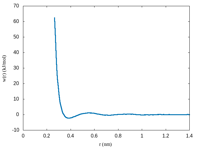
Notice that the shifted PMF goes to zero at large distances and at short distances is repulsive. At intermediate distances the potential oscillates between attractive and repulsive components corresponding to solvation shells in the liquid structure factor.

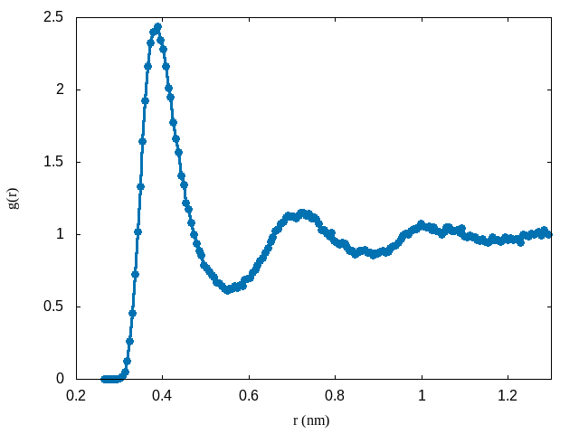
To see this, we can recall that the radial distribution function is related to the PMF according to:

Using the data from the PMF, here is a plot of the radial distribution function:

The other output from the gmx wham program is histo.xvg which shows the histogram of the sampled distances in each window. This is helpful in determining if there is enough overlap between windows. Here is a plot of each histogram for this simulation:

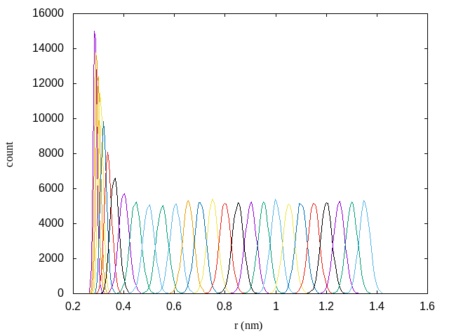
Clearly all windows are overlapping sufficiently. If there were gaps in the sampling, we could choose a smaller window size or pick specific spots that were missing to simulate.

Umbrella Sampling using PLUMED2

In this second part of the tutorial we will repeat the above example using PLUMED2 to define the reaction coordinate and perform the biasing. Here we write a plumed.dat file to define the reaction coordinate and specify the bias potential. In our plumed.dat file we have the following lines:

UNITS LENGTH=nm ENERGY=kj/mol

xi: DISTANCE ATOMS=1,6

RESTRAINT ARG=xi KAPPA=5000.0 AT=WINDOW LABEL=bias

PRINT STRIDE=200 ARG=xi,bias.* FILE=COLVAR

Here we are defining the reaction coordinate to be the distance between the methane carbons and we are using a harmonic restraint. Like before, the keyword WINDOW will be replaced in our bash script for each window. A new set of .mdp files without the COM pulling commands are available here. These are identical with the .mdp files used above, but without the COM pulling commands since we are now performing the biasing using PLUMED2.

As in the previous example, we will use a bash script to launch all the simulations. The script run-windows-umbrella-plumed.sh will replace the WINDOW keyword in the plumed.dat file and launch all the simulations for the separate windows:

#!/bin/bash
set -e

for ((i=0;i<27;i++)); do

    x=$(echo "0.05*$(($i+1))" | bc);

    sed 's/WINDOW/'$x'/g' plumed.dat > plumed.$i.dat
    gmx grompp -f mdp/min.mdp -o min.$i -pp min.$i -po min.$i
    gmx mdrun -deffnm min.$i -plumed plumed.$i.dat
    mv COLVAR COLVAR-min.$i

    gmx grompp -f mdp/min2.mdp -o min2.$i -c min.$i -t min.$i -pp min2.$i -po min2.$i -maxwarn 1
    gmx mdrun -deffnm min2.$i -plumed plumed.$i.dat
    mv COLVAR COLVAR-min2.$i

    gmx grompp -f mdp/eql.mdp -o eql.$i -c min2.$i -t min2.$i -pp eql.$i -po eql.$i
    gmx mdrun -deffnm eql.$i -plumed plumed.$i.dat
    mv COLVAR COLVAR-eql.$i

    gmx grompp -f mdp/eql2.mdp -o eql2.$i -c eql.$i -t eql.$i -pp eql2.$i -po eql2.$i
    gmx mdrun -deffnm eql2.$i -plumed plumed.$i.dat
    mv COLVAR COLVAR-eql2.$i

    gmx grompp -f mdp/prd.mdp -o prd.$i -c eql2.$i -t eql2.$i -pp prd.$i -po prd.$i
    gmx mdrun -deffnm prd.$i -plumed plumed.$i.dat
    mv COLVAR COLVAR-prd.$i

    echo 'COLVAR-prd'.$i $x '5000.0' >> metadata.dat

done

In the above script we are again simulating 27 windows from 0.05 nm to 1.3 nm in distance. The bias and coordinates from the production runs are written to the output COLVAR-prd.0, …, COLVAR-prd.27 files. The final line writes a metadata.dat file that will be used by the WHAM code.

A useful stand alone code that can perform WHAM for us is available here from the Grossfield Lab. Read the documentation, and after downloading and installing the wham code, make sure you have the executable wham in your PATH.

We will need the metadata.dat file containing the information about the coordinate files and the bias parameters for each window. This file should contain a column with the name of the COLVAR file, followed by a column with the location of the bias minimum for that simulation, and a column with the value of the spring constant, as follows:

COLVAR-prd.0  0.05 5000.0
      .
      .
      .
COLVAR-prd.22 1.15 5000.0

We execute the wham code in the terminal with:

wham 0.2 1.4 80 1e-4 298.15 0 metadata.dat fes.dat

Here the first two arguments specify the boundaries of the histogram, and the third argument is the number of bins to use in the histogram. The next argument is the tolerance followed by the temperature in Kelvin (298.15 K in this case). The next value is the padding value for periodic free energy curves which is set to 0 for aperiodic reaction coordinates. Finally we specify the name of the metadata file and the output free energy file.

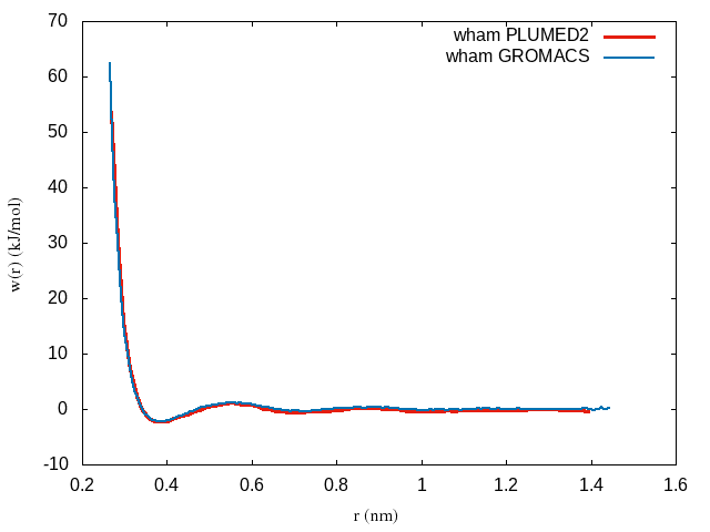
Again we can plot the output free energy as before, shifting by a constant such that the PMF goes to zero at large displacement:

plot 'fes.dat' u 1:($2+2*8.314e-3*298.15*log($1)-3.45) w l

Below is the PMF computed using the WHAM code as compared to the one we obtained above within GROMACS: