RESP fitting and partial charges for non-standard residues
About this tutorial
This tutorial demonstrates how to calculate partial charges for non-standard residues and small molecules that can be used for molecular dynamics simulations (See Protein-Ligand complex). Molecular dynamics force fields use pair-wise point charges to describe the electrostatics. Each atom has a partial charge such that the total charge on a residue is constrained to have a unit charge. For non-standard residues or small molecules, the partial charges are usually derived by performing a gas phase QM calculation. The electron density from the gas phase calculation is then fit to a classical Coulomb model with point charges on each atomic nucleus. The RESP fitting procedure uses a restraint function to fit the partial charges to the electrostatic potential.
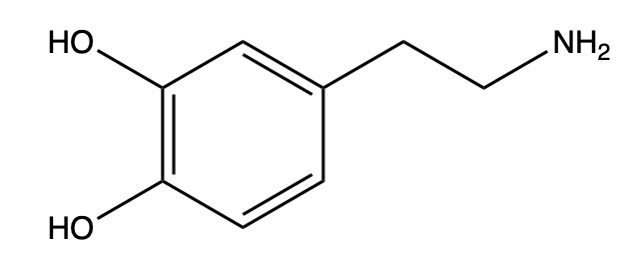
In this tutorial we will compute the partial charges for the dopamine molecule shown here:
The quantum level of theory used will be the B3LYP/6-31G* level. While more accurate ab initio methods exist, B3LYP/6-31G* gives good results for the parameterization and is widely used.
Software needed to complete this tutorial:
GAMESS-US
Orca
Open Babel
Multiwfn
Part 1: RESP fitting using GAMESS-US
In this section we use the QM software GAMESS-US to perform a geometry optimization of the structure and a single point energy calculation. We will then use the Multiwfn software to perform the RESP calculation and obtain the partial charges. We start with a pdb file for the dopamine molecule that can be made using your favorite molecular editor. An example pdb file can be found here: dopamine.pdb
First we can use OpenBabel to generate a GAMESS-US input file:
obabel -ipdb dopamine.pdb -o inp -O dopamine_opt.inpThe generated input file will look like:
$CONTRL COORD=CART UNITS=ANGS $END

$DATA
dopamine.pdb
C1
N      7.0     -0.9440000000    1.3110000000   -0.4130000000
C      6.0     -0.0690000000    2.1690000000   -1.2120000000
C      6.0      1.1060000000    1.4230000000   -1.8660000000
C      6.0      0.7110000000    0.3060000000   -2.8040000000
C      6.0     -0.0720000000    0.5600000000   -3.9450000000
C      6.0     -0.4220000000   -0.4730000000   -4.8210000000
C      6.0      0.0180000000   -1.7650000000   -4.5550000000
O      8.0     -0.2870000000   -2.8160000000   -5.3740000000
C      6.0      0.7980000000   -2.0230000000   -3.4330000000
O      8.0      1.2270000000   -3.2950000000   -3.1790000000
C      6.0      1.1520000000   -1.0030000000   -2.5610000000
H      1.0     -1.4320000000    0.6660000000   -1.0360000000
H      1.0     -0.3760000000    0.7130000000    0.1880000000
H      1.0     -0.6750000000    2.6770000000   -1.9700000000
H      1.0      0.3350000000    2.9500000000   -0.5590000000
H      1.0      1.7170000000    2.1400000000   -2.4290000000
H      1.0      1.7570000000    1.0300000000   -1.0740000000
H      1.0     -0.4120000000    1.5710000000   -4.1610000000
H      1.0     -1.0270000000   -0.2500000000   -5.6930000000
H      1.0     -0.8130000000   -2.4770000000   -6.1180000000
H      1.0      0.8540000000   -3.8270000000   -3.9090000000
H      1.0      1.7720000000   -1.2360000000   -1.6980000000
 $END
We see that the GAMESS-US format requires the atom name, the number of electrons, and the x, y, z coordinate for the atom. To perform the geometry optimization we need edit the header section of this file with the following lines:
$SYSTEM MEMDDI=400 MWORDS=200 $END
$CONTRL DFTTYP=B3LYP RUNTYP=OPTIMIZE ICHARG=0 MULT=1 COORD=CART UNITS=ANGS $END
$STATPT NSTEP=1000 $END
$BASIS GBASIS=N31 NGAUSS=6 NDFUNC=1 $END
$DATA
dopamine.pdb
C1
N      7.0     -0.9440000000    1.3110000000   -0.4130000000
C      6.0     -0.0690000000    2.1690000000   -1.2120000000
...
This sets up a geometry optimization using the B3LYP/6-31G* level of theory. The geometry optimization file is here: dopamine_opt.inp. In this example, the net charge of the molecule is 0 ICHARG=0) and the multiplicity is 1 (MULT=1). Make sure to check these values for other systems. Next we run the geometry optimization with:
rungms dopamine_opt 01 2 1 >& dopamine_opt.gmsNow we want to run a single point energy calculation and calculate the wave function for the final optimized geometry. After the job finishes, copy the optimized coordinates from the dompamine_opt.gms file into a new file called dopamine_energy.inp with the following lines:
$SYSTEM MEMDDI=400 MWORDS=200 $END
$CONTRL DFTTYP=B3LYP RUNTYP=ENERGY ICHARG=0 MULT=1 COORD=CART UNITS=ANGS $END
$BASIS GBASIS=N31 NGAUSS=6 NDFUNC=1 $END
$DATA
dopamine.pdb
C1

$END
Here we are performing a single point energy calculation. Run the single point energy calculation with:
rungms dopamine_energy 01 2 1 >& dopamine_energy.gmsWhen the calculation finishes, we perform the RESP fit using the Multiwfn software. Type:
Multiwfn dopamine_energy.gmsIn the Main function menu, select 7 Population analysis and atomic charges and then select 18 Restrained Electrostatic Potential (RESP) atomic charge. Here, we will select option 1 Start standard two-stage RESP fitting calculation
After the calculation finishes, out the atomic coordinates with charges to the file called [dopamine_energy.chg]. Looking at the this file we see the atom, x, y, z coordinate and the partial charge found by RESP fitting.
N    -3.083879    1.047791    1.080504  -0.9258644751
C    -3.230473   -0.199591    0.331421   0.4667089244
C    -2.310167   -0.386087   -0.903954  -0.2766831621
C    -0.837779   -0.412083   -0.556146   0.1721880689
C    -0.220771   -1.600247   -0.144541  -0.1761370424
C     1.125925   -1.617392    0.229820  -0.3082105594
C     1.870798   -0.443670    0.196639   0.1789935198
O     3.203835   -0.343945    0.539403  -0.5707056676
C     1.271503    0.757619   -0.216251   0.3173675689
O     1.997034    1.912630   -0.260115  -0.5221851603
C    -0.071373    0.763750   -0.585855  -0.4062687212
H    -2.114296    1.154920    1.377671   0.3439515850
H    -3.278942    1.842114    0.470928   0.3363907228
H    -3.060180   -1.029701    1.029179  -0.0474615461
H    -4.275696   -0.274588    0.004335  -0.0474615461
H    -2.588897   -1.323678   -1.404733   0.0643049079
H    -2.512089    0.423747   -1.618612   0.0643049079
H    -0.792144   -2.524995   -0.118809   0.1347340963
H     1.597625   -2.547675    0.543413   0.1641026985
H     3.539174   -1.216375    0.794707   0.4339747464
H     2.902244    1.697667    0.024127   0.4150360606
H    -0.505648    1.704084   -0.914828   0.1889200730
Part 2: RESP fitting using ORCA
As a comparison, we will also perform the QM geometry optimization using the QM software ORCA. If we use Mutiwfn to perform the RESP fit, we should obtain the same partial charges.
The ORCA input file for the geometry optimization looks like dopamine_orca_opt.inp:
!B3LYP 6-31G* TIGHTSCF Opt

%pal
nprocs 2 # parallel execution
end

* xyz 0 1
N           -0.9440000000    1.3110000000   -0.4130000000
C           -0.0690000000    2.1690000000   -1.2120000000
C            1.1060000000    1.4230000000   -1.8660000000
C            0.7110000000    0.3060000000   -2.8040000000
C           -0.0720000000    0.5600000000   -3.9450000000
C           -0.4220000000   -0.4730000000   -4.8210000000
C            0.0180000000   -1.7650000000   -4.5550000000
O           -0.2870000000   -2.8160000000   -5.3740000000
C            0.7980000000   -2.0230000000   -3.4330000000
O            1.2270000000   -3.2950000000   -3.1790000000
C            1.1520000000   -1.0030000000   -2.5610000000
H           -1.4320000000    0.6660000000   -1.0360000000
H           -0.3760000000    0.7130000000    0.1880000000
H           -0.6750000000    2.6770000000   -1.9700000000
H            0.3350000000    2.9500000000   -0.5590000000
H            1.7170000000    2.1400000000   -2.4290000000
H            1.7570000000    1.0300000000   -1.0740000000
H           -0.4120000000    1.5710000000   -4.1610000000
H           -1.0270000000   -0.2500000000   -5.6930000000
H           -0.8130000000   -2.4770000000   -6.1180000000
H            0.8540000000   -3.8270000000   -3.9090000000
H            1.7720000000   -1.2360000000   -1.6980000000
*
Here the charge and multiplicity is set by the line: xyz 0 1. Note also that we do not include the electrons, but only the atom and cartesian coordinates in the input structure. To run the optimization type:
orca dopamine_orca_opt.inp >& dopamine_orca_opt.logAgain we perform an energy minimization using the final optimized coordinates. The input file dopamine_orca_energy.inp looks like:
!B3LYP 6-31G* TIGHTSCF Energy

%pal
nprocs 2 # parallel execution
end

* xyz 0 1

*
In order to use Multiwfn with the ORCA wave function file (dopanine_orca_energy.gbw) we need to convert this file into a molden file using the orca command orca_2mkl. When the energy calculation finishes, type the following:
orca_2mkl dopamine_orca_energy -moldenThe resulting file will be a molden input file called dopamine_orca_energy.molden.input that can be loaded into Multiwfn with:
Multiwfn dopamine_orca_energy.molden.inputPerform the RESP calculation as in Part 1 and write the resulting charges to the file dopamine_orca_energy.molden.chg. The resulting charges are shown here:
N    -0.688709    1.018756   -0.181036  -0.9264440975
C    -0.157208    2.009619   -1.114961   0.4634167004
C     1.041801    1.569702   -1.996667  -0.2679759320
C     0.714522    0.421242   -2.926208   0.1644205607
C     0.139228    0.656276   -4.181416  -0.1730493830
C    -0.211046   -0.405786   -5.020941  -0.3097560636
C     0.009471   -1.716453   -4.611834   0.1802240193
O    -0.292846   -2.837758   -5.356987  -0.5712096147
C     0.586448   -1.973352   -3.357121   0.3125775736
O     0.812465   -3.255791   -2.950015  -0.5217431297
C     0.931337   -0.907959   -2.528314  -0.3970966551
H    -0.964625    0.179421   -0.689696   0.3452835040
H     0.041268    0.727898    0.469184   0.3371816829
H    -0.979849    2.327510   -1.768255  -0.0467925315
H     0.140865    2.892701   -0.534520  -0.0467925315
H     1.377239    2.436818   -2.582050   0.0619045602
H     1.877672    1.292099   -1.339669   0.0619045602
H    -0.036232    1.676476   -4.513788   0.1335915717
H    -0.651734   -0.211506   -5.997339   0.1645915383
H    -0.669125   -2.569946   -6.208720   0.4342067890
H     0.509074   -3.844506   -3.662770   0.4157840345
H     1.387982   -1.134460   -1.568880   0.1857728439
Comparing these charges to Part 1, we see that the partial charges are nearly the same.