QM/MM simulation of enzyme
Performing QM/MM hybrid simulation of chorismate mutase enzyme using CP2K and PLUMED2
About this tutorial
In this tutorial we will use the quantum chemistry code CP2K patched with PLUMED2 to setup and run a hybrid QM/MM simulation. Our model system will be the chorismate mustase enzyme that catalyzes the conversion of chorismate to prephenate. The enzyme and surrounding water will be described by classical MM force fields while the substrate is described at the QM level (using the semi-empirical PM3 method)
Summary of theory
Generally CP2K works with an additive QM/MM Hamiltonian:
\[\begin{equation}\label{EQ:E1} E^{TOT}(\textbf{R}_I,\textbf{R}_{\alpha})= E^{QM}(\textbf{R}_{\alpha}) + E^{MM}(\textbf{R}_I) + E^{QM-MM}(\textbf{R}_I,\textbf{R}_{\alpha}) \end{equation}\]where \(E^{QM}(\textbf{R}_{\alpha})\) is the pure quantum energy, \(E^{MM}(\textbf{R}_I)\) is the classical energy, and \(E^{QM-MM}(\textbf{R}_I,\textbf{R}_{\alpha})\) is a coupling term representing the mutual interaction energy of the two subsystems. These energy terms depend parametrically on the positions of the nuclei in the QM region \(\textbf{R}_{\alpha}\) and the positions of the classical atoms in the MM region \(\textbf{R}_I\).
The quantum subsystem is described at the density functional theory (DFT) level using the Quickstep algorithm. In CP2K, the classical subsystem is described through the use of the MM driver called FIST. The interaction energy term \(E^{QM-MM}(\textbf{R}_I,\textbf{R}_{\alpha})\) contains all non-bonded contributions between the QM and the MM sub-system:
\[\begin{equation}\label{EQ:E2} E^{QM-MM}(\textbf{R}_I,\textbf{R}_{\alpha}) = \sum_{I \in MM} q_I \int \frac{\rho(\textbf{r})}{|\textbf{r}-\textbf{R}_I|}d\textbf{r} + \sum_{I \in MM} \sum_{\alpha \in QM} v_{vdW}(|\textbf{R}_{\alpha}-\textbf{R}_I|) \end{equation}\]where \(\textbf{R}_I\) is the position of the MM atom a with charge \(q_I\), \(\rho(\textbf{r})\) is the total (electronic plus nuclear) charge density of the quantum system, and \(v_{vdW}\) is the van der Waals interaction between classical atom \(I\) and quantum atom \(\alpha\). The long-range electrostatic coupling contribution to the interaction energy can be classified according to the sophistication of the coupling scheme.
Embedding of QM system in MM system
Mechanical Embedding
In “mechanical embedding” schemes there is no influence of the MM charge distribution on the QM system, and the electrostatic coupling is either neglected or established using fixed effective charges to the QM nuclei, such as charges according to the MM force field. In CP2K mechanical embedding is specified by setting E_COUPL NONE
Coulomb Coupling
For semiempirical (SE) methods or DFTB we use “Coulomb” embedding where the field from the classical ions acts on the Gaussian basis functions
\[\begin{equation}\label{EQ:ECoulomb} E_{es}^{QM-MM} = - \sum_{I\in MM} ⟨\phi_a|\frac{q_I}{|\textbf{r}-\textbf{R}_I|}|\phi_b⟩ \end{equation}\]This allows for the QM region to be polarized by the MM environment. This electrostatic embedding is specified in CP2K with ECOUPL COULOMB
Gaussian Expansion of the Electrostatic Potential (GEEP)
For DFT calculations, we can use the efficient GEEP method. In this electrostatic embedding scheme, the point charge MM atoms are replaced with Gaussian charge distributions
\[\begin{equation}\label{EQ:GEEP1} \rho(|\textbf{r}-\textbf{R}_I|)=\left(\frac{1}{\sqrt{\pi}r_{c,I}}\right)\exp{\left(\frac{|\textbf{r}-\textbf{R}_I|^2}{r_{c,I}^2}\right)} \end{equation}\]where \(r_{c,I}\) is the width of the Gaussian charge of the classical atom \(I\). The electrostatic potential originated by the Gaussian charge distribution can be evaluated analytically:
\[\begin{equation}\label{EQ:GEEP2} v_I(\textbf{r},\textbf{R}_I) = \frac{erf\left(\frac{|\textbf{r}-\textbf{R}_I|}{r_{c,I}}\right)}{|\textbf{r}-\textbf{R}_I|} \end{equation}\]where \(erf(x) = \frac{2}{\sqrt{\pi}}\int_0^x e^{-t^2}\ dt\) is the error function. In GEEP, the error function is expanded as a linear combination of Gaussians and a residual function \(R_{low}\) not represented by the Gaussians, and should be rather smooth
\[\begin{equation}\label{EQ:GEEP3} v_I(\textbf{r},\textbf{R}_I) = \sum_{N_g} A_g \exp{\left( \frac{|\textbf{r} - \textbf{R}_I |^2}{r_{c,I}^2}\right)}+R_{low}(|\textbf{r}-\textbf{R}_I|) \end{equation}\]The GEEP method is specified in CP2K by setting E_COUPL GAUSS. The number of terms in the sum \(N_g\) is set by the input variable USE_GEEP_LIB. The \(A_g\) are the amplitudes of the Gaussian functions. The short range part is put onto grids in much the same manner as in the Gaussian Plane Wave (GPW) method.
Covalent Bonds Divided by the QM/MM Barrier
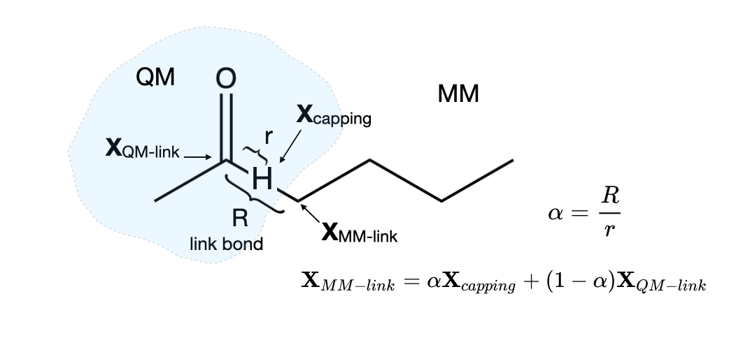
When performing a QM/MM simulation of biochemical systems, one often wants to partition the system such that some covalent bonds cross the QM/MM boundary. In this case, at least one covalent bond will involve an atom from the QM region and one from the MM region, and therefore the electronic system of the QM region must in some way be truncated as the QM/MM boundary is crossed along these so-called “link” bonds. One solutions is to introduce a “dummy atom” that caps the electronic system of the QM region. We will use the “Integrated Molecular Orbital and Molecular Mechanics” or the IMOMM method. It is important to realize that the capping atom (usually a hydrogen atom) is not part of the real system, but is simply an atom that is introduced to truncate the electronic system of the QM region. The extra degrees of freedom introduced by this extra “dummy atom” are not present in the real system. In the IMOMM method these extra degree of freedom are removed by defining the position of the MM atom that is part of the “real” link bond in terms of the QM atom it is bonded to and the capping atom that replaces it in the QM model system. Specifically, the MM link atom is constrained to lie along the bond vector of the capping atom bond, via the relation
\[\begin{equation}\label{EQ:link1} \textbf{X}_{MM-link} = \alpha \textbf{X}_{capping} + (1-\alpha)\textbf{X}_{QM-link} \end{equation}\]Where \(\textbf{X}\) refer to the Cartesian coordinates of the subscripted atoms. Since the capping atom is often at a shorter distance than the real MM atom,\(\alpha\) is usually greater than unity. For example, when a hydrogen capping atom is used to cap a C-C single bond, \(\alpha\) is around 1.38
A depiction of the relationship between the three atoms (QM-link atom, capping atom and MM-link atom) is shown below.
Preparing the Simulation Using Ambertools
Before we can run the simulation in CP2K, we will typically need to prepare the proper input files. In this case we will perform a QM/MM simulation of the chorismate mutase system. The coordinates for this system can be obtained from the protein data bank under PDB ID 2CHT.
The active complex is a trimer, forming three active sites, each of which catalyzes the reaction separately from the others. The PDB structure, however, contains twelve units with twelve inhibitors bound. We first need to remove the excess protein subunits and their inhibitors. As a first step, you can load the entire 2cht.pdb file into pymol and write only chains J, K, and L to a pdb file called protein.pdb
PyMOL> save trimer.pdb, chain J or chain K or chain LNow we will split the PDB into 5 different files: the protein, the three TSA inhibitors, and water molecules as we need to treat them separately.
grep -v -e "TSA" -e "HOH" -e "CONECT" trimer.pdb > protein.pdb
grep "TSA\ J " trimer.pdb > TSA_J.pdb
grep "TSA\ K " trimer.pdb > TSA_K.pdb
grep "TSA\ L " trimer.pdb > TSA_L.pdb
grep "HOH" trimer.pdb > waters.pdb
It is important to consider the experimental conditions we want to simulate such as the pH and salt concentration. In this case we will assume a pH=7.4. In the crystal structure all the histidines are protonated, so we need to determine the protonation state for each histidine. See Assessing the protonations states of proteins. In this case, I have changed HIS 36 and 106 in each chain to HIE (histidine protonated at the epsilon position) and HIS 54 in each chain to be in the protonated state HIP, and saved a version of the pdb file that can be used in Ambertools as protein-amber.pdb.
In addition, before we can parameterize the ligand, we need to replace the inhibitors bound to the crystal structure with copies of the substrate, chorismate. This can be done using a molecular editor. A pdb file for each ligand was prepared for you using the Jmol editor. These files are named LigandA.pdb, LigandB.pdb, and LigandC.pdb.
We will now use the antechamber and parmchk2 tools from Ambertools to generate Amber force fields for our system. For the ligands we will use the “general Amber force field 2” (GAFF2) parameters. To assign partial charges we will use the AM1-bcc method. Remember that during production runs the ligands will be in the QM region and so we do not need to worry too much about the limitations of the AM1-BCC2 method of determining the partial charges since this is used only during the equilibration stages. Since the active complex has three ligands, we will perform this parameterization for each of them:
for i in A B C; do antechamber -i Ligand${i}.pdb -fi pdb -o Ligand${i}.mol2 -fo mol2 -c bcc -nc -2 -rn CH${i} -at gaff2 -pf yes -j 5; done
for i in A B C; do parmchk2 -i Ligand${i}.mol2 -f mol2 -o Ligand${i}.frcmod -s 2; done
Here the -c bcc signals to use the AM1-BCC2 charge method, the net charge of the ligand is set with -nc -2, the name of the new residue we are generating is -rn CHA/CHB/CHC and we are spcifying to use the GAFF2 force field (-at gaff2). The parmchk2 tool checks the parameter file for possible missing firce field parameters and generates a parameter file that can be loaded into Leap in order to add these missing parameters. If possible, it will fill in the missing parameters by analogy to similar parameters. You should check these parameters before running a simulations. In the case where antechamber cannot empirically calculate a value or has no analogy it will add the comment: “ATTN: needs revision.” In this case you will have to manually parameterize this yourself.
We now can build the system with tLEap. First we load the default force fields (amberff14SB, tip3p, and GAFF2):
# Load force field parameters
source leaprc.protein.ff14SB
source leaprc.gaff2
source leaprc.water.tip3p
Now we load our three ligand moleucles, our protein, and water molecules:
# Load extraparameters for the ligand
loadamberparams LigandA.frcmod
loadamberparams LigandB.frcmod
loadamberparams LigandC.frcmod

# Load protein, ligand and water molecules
protein = loadPDB protein-amber.pdb
LigA = loadmol2 LigandA.mol2
LigB = loadmol2 LigandB.mol2
LigC = loadmol2 LigandC.mol2
waters = loadPDB waters.pdb
Now we join all these pieces of our system into one with the combine command:
# Build system
system = combine {protein LigA LigB LigC waters}
savepdb system system.dry.pdb

check system
It is good practice to save a pdb of your system with the savePDB command and to perform a quick check of your system with the check command. At this stage, it is normal to have warnings for close contacts between atoms since we have added hydrogens and to have a net charge on the molecule since we have not added counter ions. If the final line is “Unit is OK,” we can continue. Now we need to solvate our system and add counter ions to neutralize our system.
# Solvate
solvateBox system TIP3PBOX 14 iso

# Neutralize
addIonsRand system Na+ 0
Here we have set the size around our protein as 14 nm and specify to use a cubic box with the iso flag. Now we can save our topology and coordinates file with saveamberparm.
# Save Amber input files
savePDB system system.pdb
saveAmberParm system system.parm7 system.rst7

quit
All of the above commands are provided in a leapin file. To execute it, you can type the following:
tleap -f leapinEnergy minimization at the MM level
Before moving to CP2K, we will first minimize our system using the sander tool fro AmberTools. To run sander, one needs to specify the initial coordinates (-c system.rst7) and the topology file (-p system.parm7) and an input file containing the details of the minimization (-i sander_min.in). For our energy minimization, we will perform 4000 steps using two different methods: 2000 of gradient descent and 2000 of conjugate gradient. The sander input file looks like:
Minimization of system
 &cntrl
  imin=1,         ! Perform an energy minimization
  maxcyc=4000,    ! The maximum number of cycles of minimization
  ncyc=2000,      ! The method will be switched from steepest descent to conjugate gradient after NYCY cycles
/
Run the minimization by executing the following command:
sander -O -i sander_min.in -o min_classical.out -p system.parm7 -c system.rst7 -r system.min.rst7This will take a while. You can watch the progress of the minimization by typing
tail -f min_classical.outFinally, we convert the output restart file to an input coordinate file that can be read by CP2K using cpptraj. First load the topology file:
cpptraj -p system.parm7Then, we provide an input trajectory with trajin
trajin system.min.rst7
trajout system.min0.rst7 inpcrd
go
quit
We now have a topology file system.parm7 and energy minimized coordinates file system.min.0.rst7 that we can use in CP2K.
We will first run a quick energy minimization in CP2K. The CP2K input file cp2k_em.inp contains the information for our equilibration. A CP2K input is divided into different sections. The first section is the &GLOBAL section that contains general information regarding the kind of simulation to perform. Here we specify that we will do a geometry optimization (energy minimization) and set the output verbosity to low.
&GLOBAL
  PROJECT EM
  PRINT_LEVEL LOW
  RUN_TYPE GEO_OPT
&END GLOBAL
The next section is the &FORCE_EVAL section that contains the parameters needed to calculate the energy and forces. Molecular mechanics in CP2K is performed using the FIST algorithm:
&FORCE_EVAL
  METHOD FIST
  ...
Next, within the &FORCE_EVAL section we have the subsection &MM which includes the parameters to run a MM calculation. Here we specify to use the Amber force fields and to use our input topology file system.parm7. We specify how to handle the long-range electrostatics using the Ewald Summation method in the &POISSON subsection. Here we specify to use the smooth particle mesh using beta-Euler spines (SPME) method.
...
 &MM
  &FORCEFIELD
    PARMTYPE AMBER
    PARM_FILE_NAME system.parm7
    &SPLINE
      EMAX_SPLINE 1.0E8
      RCUT_NB [angstrom] 10
    &END SPLINE
  &END FORCEFIELD
  &POISSON
     &EWALD
      EWALD_TYPE SPME
      ALPHA .40
      GMAX 80
     &END EWALD
  &END POISSON
&END MM
...
The next subsection is &SUBSYS which specifies the information of the system box size and coordinates. It is very important to use the current size of your simulation box in &FORCE_EVAL > &SUBSYS > &CELL. To get this information, you can type the following:
tail -1 system.min0.rst7and add the X Y Z values in the ABC section and alpha beta gamma to the ALPHA_BETA_GAMMA section.
...
  &SUBSYS
    &CELL
      ABC [angstrom] 87.7209030 87.9216130 87.672390
      ALPHA_BETA_GAMMA 90 90 90
    &END CELL
    &TOPOLOGY
      CONN_FILE_FORMAT AMBER
      CONN_FILE_NAME system.parm7
      COORD_FILE FORMAT CRD
      COORD_FILE_NAME system.min0.rst7
    &END TOPOLOGY
    !Na+ is not recognized by CP2K, so it is necessary to define it here using KIND
    &KIND Na+
      ELEMENT Na
    &END KIND
  &END SUBSYS
&END FORCE_EVAL
For an energy minimization run we include the section &MOTION to specify the parameters for the geometry optimization:
&MOTION
  &GEO_OPT
   OPTIMIZER LBFGS
   MAX_ITER 1000
   MAX_DR 1.0E-02
   RMS_DR 5.0E-03
   MAX_FORCE 1.0E-02
   RMS_FORCE 5.0E-03
  &END
...
The full CP2K energy minimization file cp2k_em.inp is provided. Run this using CP2K:
cp2k.sopt cp2k_em.inp > em.outFirst, check the em.out file for any warnings. In this case we have 2 warnings. The first warning is about missing forcefield terms. You could print this information using &FORCE_EVAL > &MM > &PRINT > &FF_INFO. In this case the non-critical missing terms are Urey-Bradley interactions which are not used in the Amber force fields, so we can ignore this warning. A second warning is that our CRD file lacks velocities and box information will not be read. This warning is not a problem either, since we do not have velocities yet, and box parameters were provided in the CP2K input file. At this stage you should also visualize the output structure file EM-pos-1.pdb to make sure nothing looks weird with the simulation box.
Equilibration at the MM level using CP2K
After the energy minimization step, we will equilibrate the temperature using a 5 ps classical MD simulations in the NVT ensemble. The CP2K input file for this run is called cp2k_equil_nvt.inp. One difference between this input file and the previous energy minimization file is that the &GLOBAL section now specifies that the RUN_TYPE will be MD
&GLOBAL
  PROJECT NVT
  PRINT_LEVEL LOW
  RUN_TYPE MD
&END GLOBAL
The main difference between this file and the previous energy minimization run is the &MD section which tells CP2K how to move the atomic nuclei. Here we are performing a MD simulation in the NVT ensemble.
&MOTION
  &MD
  ENSEMBLE NVT
  TIMESTEP [fs] 0.5
  STEPS 10000
  TEMPERATURE 298
  &THERMOSTAT
    REGION GLOBAL
    TYPE CSVR
    &CSVR
      TIMECON [fs] 10.
    &END CSVR
  &END THERMOSTAT
 &END MD
In the above command we have specified the thermostat as canonical sampling through velocity rescaling with the &CSVR section. We will use our previous energy minimization restart file as the input coordinates specified with the &EXT_RESTART section
&EXT_RSTART
  RESTART_FILE_NAME EM-1.restart
  RESTART_DEFAULT .FALSE.
  RESTART POS TRUE
&END
Have a look at the cp2k_equil_nvt.inp input file to make sure you understand what each section does. Then run the simulation with
cp2k.sopt cp2k_equil_nvt.inp > nvt.outThe output file NVT-1.ener contains information about the energy and temperature during the simulation and can be used to check that the temperature is properly equilibrated.
After the NVT simulation has completed, we will perform a 50 ps NPT equilibration to let the pressure and density equilibrate by allowing the box volume to fluctuate. The CP2K input file for this run is called cp2k_equil_npt.inp. The main addition to this file from before is the introduction of a barostat to the &MD section:
&BAROSTAT
  TIMECON [fs] 100
  PRESSURE [bar] 1.0
&END BAROSTAT
After looking at the cp2k_equil_npt.inp input file, run the NPT simulation with
cp2k.sopt cp2k_equil_npt.inp > npt.outAt the end of this NPT equilibration we are now ready to move to a QM/MM simulation. Make sure to update your CP2k input files to use the final equilibrated box coordinates from the NPT equilibration. The cell dimensions are printed in the NPT-1.cell file.
Adding missing LJ parameters
In the classical Amber MM forcefields, some hydrogen atoms do not have Lennard-Jones parameters. Before running any QM/MM simulation, we need to provide these parameters. We are going to add the values of the hydrogen atom that corresponds to the hydroxyl (alcohol group) in the GAFF forcefield to TIP3P water (:WAT@H1 and :WAT@H2) and to the hydroxyl groups from serine (:SER@HG), tyrosine (:TYR@HH), and threonine (:THR@HG1) residues. (threonine).
To do this we will use the parmed tool of the Ambertools package. First load the topology file:
parmed system.parm7We can check if there are missing parameters by printing an atom index (5724 corresponds to the hydrogen atom on the first water molecule) using the printDetails command:
printDetails @5724 which gives as the output
The mask @5724 matches 1 atoms:

 ATOM  RES  RESNAME  NAME  TYPE  At.#  LJ Radius  LJ Depth    Mass  Charge  GB Radius  GB Screen
 5724  364      WAT    H1    HW     1     0.0000    0.0000  1.0080  0.4170     0.8000     0.8500
Here we see that the LJ Radius and LJ Depth values are set to 0. To see similar details for all the HO group hydrogens:
printDetails @%HO It is important to modify these missing parameters before running a QM/MM simulation to prevent unphysical interacts between the hydrogen atoms without LJ parameters and the QM subsystem. After this topology correction, the thermostat should stay stable during the QM/MM calculation. We use the changeLJSingleType command on different atom types to modify the force field parameters:
changeLJSingleType :WAT@H1 0.3019 0.047
changeLJSingleType :WAT@H2 0.3019 0.047
changeLJSingleType :SER@HG 0.3019 0.047
changeLJSingleType :TYR@HH 0.3019 0.047
changeLJSingleType :THR@HG1 0.3019 0.047
which gives as the output
Changing :WAT@H1 Lennard-Jones well depth from 0.0000 to 0.0470 (kcal/mol) and radius from 0.0000 to 0.3019 (Angstroms)
...
Finally, we save a new topology using the command outparm and exit
outparm system_LJ_mod.parm7
quit
You can also run parmed with the provided input file parmed.in
parmed system.parm7 -i parmed.inQM/MM in CP2K
Usually, we will want to include relevant side chain amino acids in the QM region and link them to the MM region as described above. In the classical amber force fields, each atom is given a partial charge and the sum over all the partial charges equal the total charge on the residue. For example in Arg90 of our system, the total partial charges sum up to +1. When we move a side chain to the QM region, the QM calculation will always distribute a whole (integer) charge over all atoms (QM atoms plus a link atom). If the sum of partial charges of the atoms that were moved to the QM region is not initially a whole number, it will be forced into a whole number after the first QM step, where the charge of the link atom is distributed over the QM region. This will create a mismatch between QM and MM charges, changing the total charge of the entire system (QM plus MM regions). An example of Arg90 is shown here:
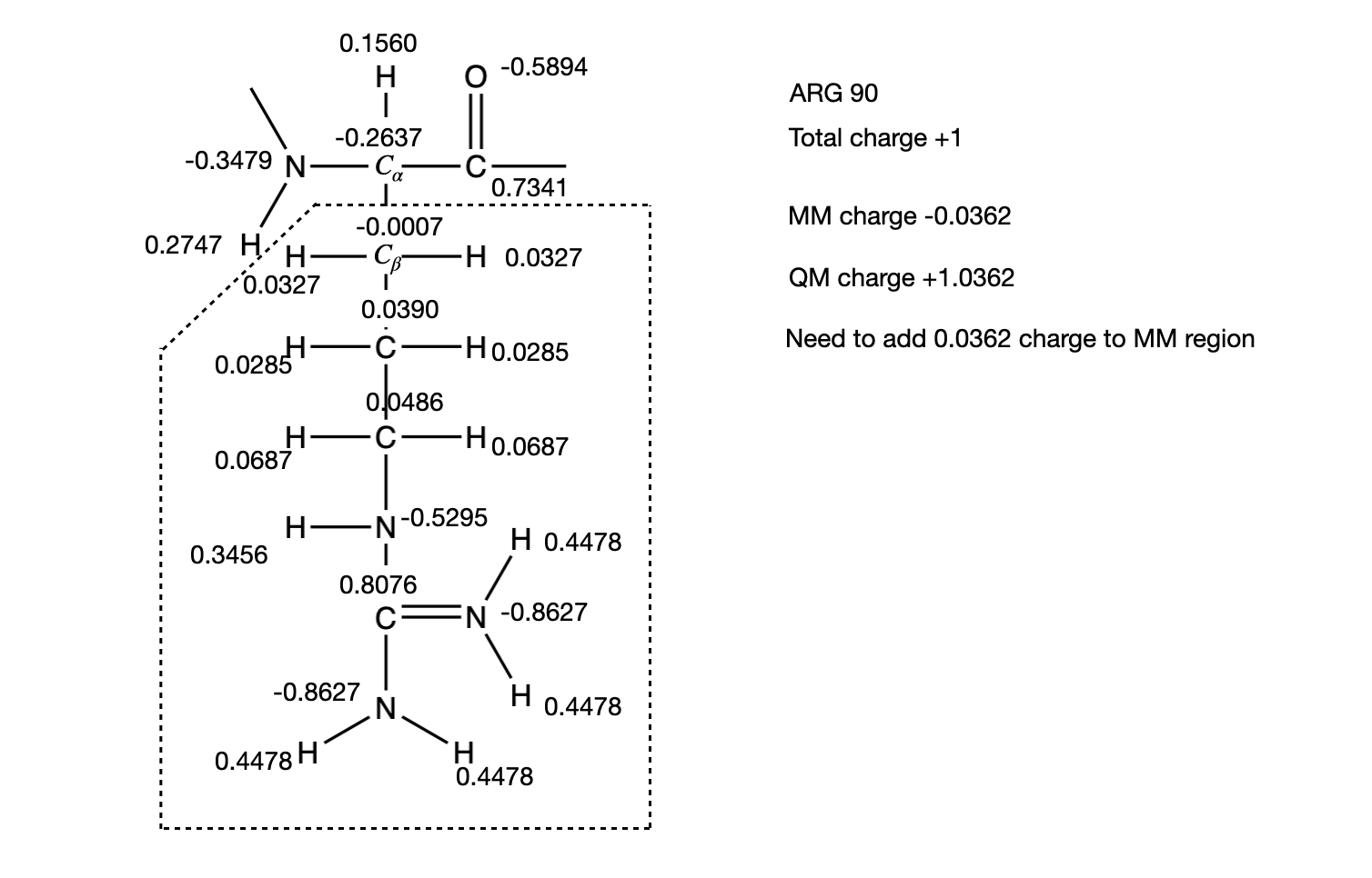
If the bond between \(C_\alpha\) and \(C_\beta\) is chosen for the link bond, the charge of the MM region would be -0.0362, while the charge of the QM region would be 1.0362. Since the QM calculation would place a pre-determined whole charge on the region (+1, in this case), the updated charge of the QM region after the first simulation step would change the total charge of the system to -0.0362, in this example. We can neutralize the MM region of the system by distributing an equal but opposite charge across the 6 main chain atoms of the residue in the MM region. For example the charge on the N is -0.3479. Adding 0.0362/6 to this value gives a new charge on the N atom of -0.3419. We can repeat this calculation for the remaining main chain atoms and check that the modified charges on the MM region add up to zero. Open parmed as before:
parmed system_LJ_mod.parm7and apply the changes to the 6 main chain atoms:
change charge @1409 -0.3419
change charge @1410 0.2807
change charge @1411 -0.2577
change charge @1412 0.1620
change charge @1431 0.7401
change charge @1432 -0.5834
outparm system_qm-charge.parm7
quit
When we move from MM to QM/MM hybrid simulations, the main changes are that we need to specify how the QM region will be handled in the &FORCE_EVAL section. We specify the electronic structure method to be employed by the QUIKSTEP algorithm within the &QS section. In this example, we specify the PM3 semiempirical method with a cutoff for the evaluation of the Coulomb term and the Exchange integrals in the SE calculation of 10.0 Angstroms. We also set the parameters needed to perform the SCF run within the &SCF section.
&FORCE_EVAL
   METHOD QMMM
   STRESS_TENSOR_ANALYTICAL
   &DFT
     CHARGE -1
     &QS
       METHOD PM3
       &SE
         &COULOMB
           CUTOFF [angstrom] 10.0
         &END
         &EXCHANGE
           CUTOFF [angstrom] 10.0
         &END
       &END
     &END QS
     &SCF
       MAX_SCF 30
       EPS_SCF 1.0E-6
       SCF_GUESS ATOMIC
       &OT
         MINIMIZER DIIS
         PRECONDITIONER FULL_SINGLE_INVERSE
       &END
       &OUTER_SCF
         EPS_SCF 1.0E-6
         MAX_SCF 10
       &END
      &END SCF
    &END DFT
...
Notice that the charge in the QM system has been set to -1 with CHARGE -1 in the &DFT section. The chorismate enzyme has a total charge of -2 and we have added a +1 charge due to the addition of the Arg90 side chain to the QM region.
We will also have to specify how to embed the QM system and which atoms should be treaded at the QM level using the &QM_KIND section. For semiempirical methods we can use Coulombic electrostatic embedding. Here we include all the atom indices for the chorismate molecule and Arg90 side chain atoms from the topology file.
...
   &QMMM
     ECOUPL COULOMB
     &CELL
        ABC 40 40 40
        ALPH_BETA_GAMMA 90 90 90
     &END CELL
     &QM_KIND  H
      MM_INDEX 5663
      MM_INDEX 5664
      MM_INDEX 5665
      MM_INDEX 5666
      MM_INDEX 5667
      MM_INDEX 5669
      MM_INDEX 5670
      MM_INDEX 5686
      MM_INDEX 1414
      MM_INDEX 1415
      MM_INDEX 1417
      MM_INDEX 1418
      MM_INDEX 1420
      MM_INDEX 1421
      MM_INDEX 1423
      MM_INDEX 1426
      MM_INDEX 1427
      MM_INDEX 1429
      MM_INDEX 1430
    &END QM_KIND
    &QM_KIND  C
      MM_INDEX 5668
      MM_INDEX 5671
      MM_INDEX 5673
      MM_INDEX 5675
      MM_INDEX 5677
      MM_INDEX 5679
      MM_INDEX 5681
      MM_INDEX 5683
      MM_INDEX 5684
      MM_INDEX 5685
      MM_INDEX 1413
      MM_INDEX 1416
      MM_INDEX 1419
      MM_INDEX 1424
    &END QM_KIND
    &QM_KIND  O
      MM_INDEX 5672
      MM_INDEX 5674
      MM_INDEX 5676
      MM_INDEX 5678
      MM_INDEX 5680
      MM_INDEX 5682
    &END QM_KIND
    &QM_KIND  N
      MM_INDEX 1422
      MM_INDEX 1425
      MM_INDEX 1428
    &END QM_KIND
    &LINK
      MM_INDEX  1411
      QM_INDEX  1413
      LINK_TYPE IMOMM
      ALPHA_IMOMM 1.38
    &END LINK
  &END QMMM
&END FORCE_EVAL
Notice that here we need to specify how to link the QM and MM subsystems. In this case we create a link between MM atom 1411 \((C_\alpha)\) and QM atom 1413 \((C_\beta)\) and we specify to use the IMOMM method for the link. The CP2K input file for this run is called cp2k_monitor.inp This will perform a 5 ps QM/MM simulation in the NVT ensemble. After looking at this file to make sure you understand what parameters are being set, you can run the QM/MM simulation as:
cp2k.sopt cp2k_monitor.inp > monitor.outThe output trajectory file is MONITOR-1.pos.dcd. If you look at the trajectory using VMD, you will see that no reaction occurred in this short amount of time. This is because of the significant energy barrier that must be overcome for the reaction to occur.
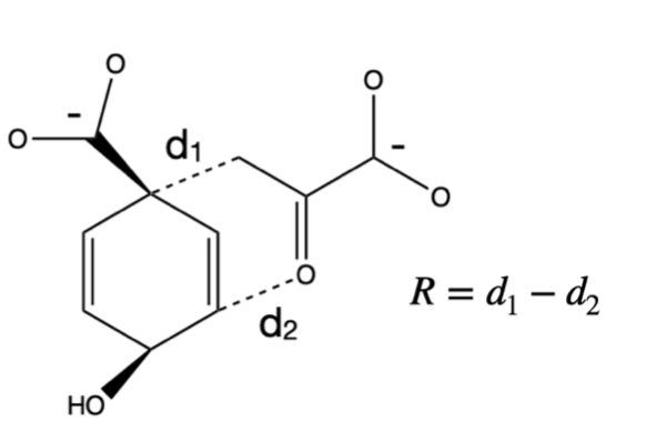
If CP2K is patched with plumed, we can monitor the time series of a collective variable. In this case we define the difference between the C-O bond distance (\(d_2\)) that will be breaking and the C-C bond (\(d_1\)) that will be forming as shown below:
Create a file called plumed-monitor.dat with the following:
UNITS LENGTH=A TIME=fs ENERGY=kcal/mol
WHOLEMOLECULES ENTITY0=1-5711

d1: DISTANCE ATOMS=5668,5671
d2: DISTANCE ATOMS=5682,5679

COMBINE ARG=d1,d2 COEFFICIENTS=1,-1 PERIODIC=NO LABEL=zeta

PRINT ARG=d1,d2,zeta FILE=COLVAR STRIDE=10
FLUSH STRIDE=10
In the above we are monitoring the C-C bond distance, the C-O bond distance, and the difference between them, and we are printing these values to the COLVAR file every 10 steps.
Now we need to add a &FREE_ENERGY section to the cp2k_monitor.inp file under the &MOTION section:
&MOTION
...
 &FREE_ENERGY
   &METADYN
      USE_PLUMED .TRUE.
      PLUMED_INPUT_FILE ./plumed-monitor.dat
   &END METADYN
&END FREE_ENERGY
Metadynamics using PLUMED2
In order to observe the reaction in a reasonable amount of computational time, we will use metadynamics to bias the CV and explore new regions of CV space. To implement metadynamics, add the following lines to your plumed file and save the file as plumed.dat
METAD ...
   ARG=zeta
   HEIGHT=1.5
   SIGMA=0.2
   PACE=100
   LABEL=bias
... METAD
Here we set the Gaussian hill height to 1.5 kcal/mol and the Gaussian width to be 0.2 Angstroms. A new Gaussian biasing kernel will be deposited every 100 steps.