Born Oppenheimer simulation of liquid water
About this tutorial
In this tutorial we perform a simulation of bulk liquid water using the quantum chemistry code CP2K. This system is well-studied and often used as a benchmark for ab initio MD (AIMD) simulations. For example, you should take a look at the reference J. Phys. Chem. B 2009, 113, 35, 11959–11964. The syntax for the CP2K input file from this tutorial can be used as a starting point for other ab initio MD simulations in CP2K with modifications as needed.
Summary of theory
In quantum mechanics both the electrons and nuclei are described using the time-dependent Schrödinger equation
\[\begin{equation}\label{EQ:SE} i \hbar \frac{\partial \Psi(r_i, R_I,t)}{\partial t} = H \Psi(r_i,R_I,t) \end{equation}\]with
\[\begin{equation}\label{EQ:Htotal} H = -\sum_I \frac{\hbar^2}{2M_I}\nabla_I^2 + H_e \end{equation}\] \[\begin{equation}\label{EQ:He} H_e = -\sum_i \frac{\hbar^2}{2m_e}\nabla_i^2 + \frac{1}{4\pi \epsilon_0}\sum_{i<j} \frac{e^2}{|\textbf{r}_i-\textbf{r}_j|} - \frac{1}{4\pi \epsilon_0}\sum_{I,i} \frac{e^2 Z_I}{|\textbf{R}_I-\textbf{r}_i|} + \frac{1}{4\pi \epsilon_0}\sum_{I<J} \frac{e^2Z_IZ_J}{|\textbf{R}_I-\textbf{R}_J|} \end{equation}\]where \(\textbf{R}_I\) is the atomic position, \(Z_I\) is the atomic charge, \(M_I\) is the atomic mass, \(\textbf{r}_i\) is the electron position and \(m_e\) is the electron mass.
In Born-Oppenheimer MD (BOMD) only the ground state wave function is included and the wave function is assumed to be always at the minimum. The BOMD equations of motion are thus:
\[\begin{equation}\label{EQ:BOMD} M_I \frac{d^2\textbf{R}_I(t)}{dt^2} = -\nabla_I \min_{\Psi_0}\left< \Psi_0 | H_e | \Psi_0\right> \end{equation}\] \[\begin{equation}\label{EQ:BOMD2} E_0 \Psi_0 = H_e \Psi_0 \end{equation}\]where we note that \(H_e\) depends on the atomic positions. The next step is to solve the electronic Schrödinger equation using some level of approximation like Hartree-Fock (HF) or Density Functional Theory (DFT). AIMD simulations are very computationally expensive as compared to classical molecular dynamics (MD) but have the great advantage of allowing for chemical bonds to break and form. Furthermore, with a suitable choice of basis set and pseudopotentials, the numerical approximations are small and these methods can be quite accurate.
DFT in CP2K is performed using the Quickstep code that uses a Gaussian and plane waves (GPW) method.
AIMD of bulk liquid water
In this section we will perform Born-Oppenheimer MD of bulk liquid water containing 64 water molecules (192 atoms) in a 12.42 Å\(^3\) box. The starting configuration water.xyz is in xyz format and available here. The other file we need is a CP2K input file water.inp. A CP2K input file is divided into sections. The section &GLOBAL contains general information regarding the kind of simulations to perform and any global parameters. In our file we have specified the run-type to be MD (molecular dynamics) and set the output verbosity to low.
&GLOBAL
   PROJECT WATER
   RUN_TYPE MD
   PRINT_LEVEL LOW
&END GLOBAL
Next, we define the parameters needed to calculate the energy and forces with the &FORCE_EVAL section. In BOMD the forces come from the solution of the electronic Schrödinger equation. First we specify the method we are using to compute the forces as QUICKSTEP
&FORCE_EVAL
METHOD QUICKSTEP
The we need to specify the parameters need by the LCAO DFT program. In the tutorial we will use the DZVP-GTH-BLYP basis set found in the file BASIS_SET located in cp2k/data and we will use the pseudopotential of Goedecker, Teter, and Hutter (GTH) located in the POTENTIAL file in cp2k/data. We set the planewave cutoff to 340 Ry
&DFT
BASIS_SET_FILE_NAME BASIS_SET
POTENTIAL_FILE_NAME POTENTIAL
&MGRID
   CUTOFF 340
   REL_CUTOFF 50
&END MGRID
Next, we specify the parameters to uses in the QUIKSTEP framework with the &QS section. We set the electronic structure method as GPW (Gaussian and plane waves method) and the ASPC stable predictor corrector for MD stability.
&QS
METHOD GPW
EPS_DEFAULT 1.0E-10
EXTRAPOLATION ASPC
&END
For systems with periodic boundary conditions (condensed phases) we specify the directions in which PBC applies for the electrostatics with the &POISSON section:
&POISSON
   PERIODIC XYZ
&END
Now we set the parameters needed to perform the SCF run with the %SCF section. Our initial guess is the atomic wavefunction, and we set the target accuracy for SCF convergence and maximum number of SCF iterations. The subsection &OT sets the various options for the orbital transformation (OT) method. The OT method is a direct minimization scheme that allows for efficient wave function optimization for large systems.
&SCF
  SCF_GUESS ATOMIC
  MAX_SCF 30
  EPS_SCF 1.0E-6
  &OT
   PRECONDITIONER FULL_ALL
   MINIMIZER DIIS
  &END OT
&END SCF
Next for performing the DFT calculation we need to specify the exchange correlation potential. We specify the parameters for the exchange correlation potential in the section &XC. In this tutorial we will use the BLYP functional
&XC
  &XC_FUNCTIONAL BLYP
  &END_XC_FUNCTIONAL
&END XC
Lastly we specify the print options for the DFT part of the code with the &PRINT section and then end the &DFT section
&PRINT
  &E_DENISTY_CUBE
  &END E_DENSITY_CUBE
&END PRINT
&END DFT
After specifying the DFT section, we specify the subsystem coordinates, topology, and cell size with the &SUBSYS section. We specify the unit cell dimensions (in Angstroms) with the &CELL section. Next we specify the atomic coordinates in XYZ format. Finally, we specify the basis set and pseudopotential to use for each atom type and the end the &FORCE_EVAL section
&SUBSYS
  &CELL
    ABC [angstrom] 12.42 12.42 12.42
  & END CELL

  &TOPOLOGY
    COORD_FILE_NAME water.xyz
    COORD_FILE_FORMAT XYZ
  &END TOPOLOGY

  &KIND O
    BASIS_SET DZVP-GTH-BLYP
    POTENTIAL GTH-BLYP-q6
  &END KIND
  &KIND H
    BASIS_SET DZVP-GTH-BLYP
    POTENTIAL GTH-BLYP-q1
  &END KIND
&END SUBSYS
&END FORCE_EVAL
In the section &MOTION we define the molecular dynamics parameters for propagating the atomic coordinates (nuclei). We are performing molecular dynamics in the NVT ensemble. We set the time step for the equation of motion to 0.5 fs. The temperature will be controlled by the velocity rescaling thermostat.
&MOTION
&MD
  ENSEMBLE NVT
  TEMPERATURE 300
  TIMESTEP 0.5
  STEPS 1000
  &THERMOSTAT
    TYPE CSVR
    &CSVR
      TIMECON 1.0
    &END CSVR
  &END THERMOSTAT
&END MD
Finally, before we end the &MOTION section we will specify what properties of the MD run to print and how often.
&PRINT
  &TRAJECTORY
    &EACH
      MD 10
    &END EACH
  &END TRAJECTORY
  &VELOCITIES OFF
  &END VELOCITIES
  &FORCES OFF
  &END FORCES
  &RESTART_HISTORY
    &EACH
      MD 5000
    &END EACH
  &END RESTART_HISTORY
  &RESTART
    BACKUP_COPIES 3
  &EACH
    MD 10
  &END EACH
  &END RESTART
&END PRINT
&END MOTION
Once you understand the input file water.inp, you are now ready to run the simulation
cp2k.popt water.inpAnalyzing Results
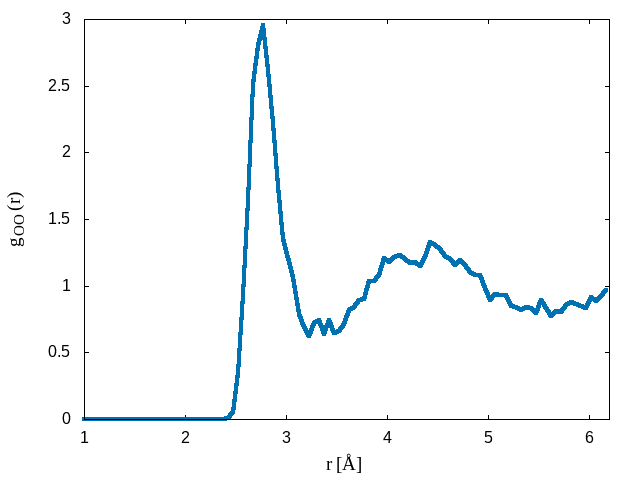
The trajectory file WATER-pos-1.xyz is in xyz format and can be viewed using programs like Molden or VMD. See if you can create a representation that shows the dynamic hydrogen bond network. The python script calc_gofr.py will compute the radial distribution function between atoms given a trajectory in xyz format. To run the script type:
python calc_gorf.py -i WATER-pos-1.xyz -atom1 O -atom2 O -box 12.42 -o grOO.datThe above script will calculate the radial distribution function between pairs of oxygen atoms. The peak in the O-O radial distribution function occurs at roughly 2.8 Å which is the well known average hydrogen bond length in water.
A plot of the radial distribution function \(g_{OO}(r)\) is shown below:
The other output file is the .ener file WATER-1.ener that contains information about the energy and temperature during the simulation. Using gnuplot compare columns 4,5 and 6 which are the temperature, potential energy, and conserved quantity.
gnuplot> plot 'WATER-1.ener' u 2:4 w lp
gnuplot> replot 'WATER-1.ener' u 2:5 w lp
gnuplot> replot 'WATER-1.ener' u 2:6 w lp
Hydronium ion
The structure file hydronium.xyz contains a single hydronium ion in a system with 5 other water molecules. We can run the simulation as before, except that now the total charge of the system is +1. Modify the water.inp file such that
CHARGE 1
MULTIPLICITY 1
We have also made the system smaller to speed up the calculation, so we need to update the box size accordingly and make sure the input coordinate file is specified to hydronium.xyz:
&CELL
  ABC [angstrom] 7.83 7.83 7.83
&END CELL

&TOPOLOGY
  COORD_FILE_NAME hydronium.xyz
  COORD_FILE_FORMAT XYZ
Now, run the simulation as before:
cp2k.popt water.inpWhen the simulation finishes, see if you can visualize the Grotthuss mechanism