McCarty Group Wiki

Analyzing a MD Trajectory

About this tutorial

This tutorial deals with extracting basic information from a MD trajectory performed in GROMACS. If you have not yet completed the Basics of a GROMACS simulation, you should do that tutorial before proceeding to this tutorial. This tutorial will introduce you to a few basic tools to analyze a generated trajectory. In this tutorial we will analyze the ubiquitin simulation from before. For your own system, you should formulate for yourself some ideas about the types of data you will want to collect.

Converting trajectory formats

The Gromacs command trjconv is a post-processing tool to manipulate the atomic coordinates, extract a subset of the coordinates, correct for periodic boundary conditions (pbc), or manually alter the trajectory (time units, frame frequency, etc.). Here we will correct for the periodicity of the system. The protein will diffuse through the unit cell and may appear to “jump” across to the other side of the box. To account for such actions, apply the following command:

$ gmx trjconv -s md_trajectory.tpr -f md_trajectory.xtc -o md_trajectory_noPBC.xtc -pbc whole -ur compact

where -s signals the input .tpr file that was used to run the MD simulation (here called md_trajectory.tpr) and -f signals the trajectory that was produced by the GROMACS mdrun command. Here we are using the compressed .xtc format. The -o is the output modified trajectory file. The -pbc whole flag signals to make molecules that were split by the periodic boundary conditions whole and the -ur compact flag signals to keep all molecules in the original unit cell. When prompted select option 0 for the entire system.

In the remainder of this tutorial we will work with this “corrected” trajectory md_trajectory_noPBC.xtc

If you want to look at a movie of the whole trajectory, you can convert the xtc file to a pdb file using trjconv command

$ gmx trjconv -s md_trajectory.tpr -f md_trajectory_noPBC.xtc -o md.pdb

This will convert the trajectory into .pdb format which can be viewed in PyMOL or VMD.

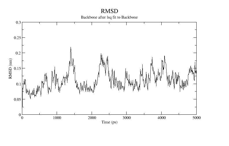
Root-mean-square deviation (RMSD) of atomic positions

The root-mean-square deviation of atomic positions (or simply root-mean-square deviation, RMSD) is the measure of the average distance between the atoms (usually the backbone atoms) of superimposed proteins. This will give a measure of the overall change in the conformation of the protein as the rmsd with respect to a reference state. We can use the first frame of the trajectory as a reference state. First we will extract this frame using trjconv

$ gmx trjconv -s md_trajectory.tpr -f md_trajectory.xtc -o frame1.pdb -pbc whole -ur compact -dump 0

where we again correct for periodic boundary conditions as before, but here we output just the first frame with the flag -dump 0.

To compute the RMSD enter the command:

$ gmx rms -s frame1.pdb -f md_trajectory_noPBC.xtc -o rmsd-vs-start.xvg

First the algorithm will align each structure to the reference configuration (frame1.pdb). We must select which atoms to use for the least-squares aliment. Common choices include the backbone atoms or all heavy atoms. When prompted, select 4 for Backbone atoms. The next prompt will ask us to select a group for the RMSD calculation. You can again experiment with different selections. Here we will select 4 again for the Backbone atoms.

Plot the generated rmsd-vs-start.xvg using the Xmgrace plotting tool

xmgrace rmsd-vs-start.xvg

A plot of the RMSD is shown below:

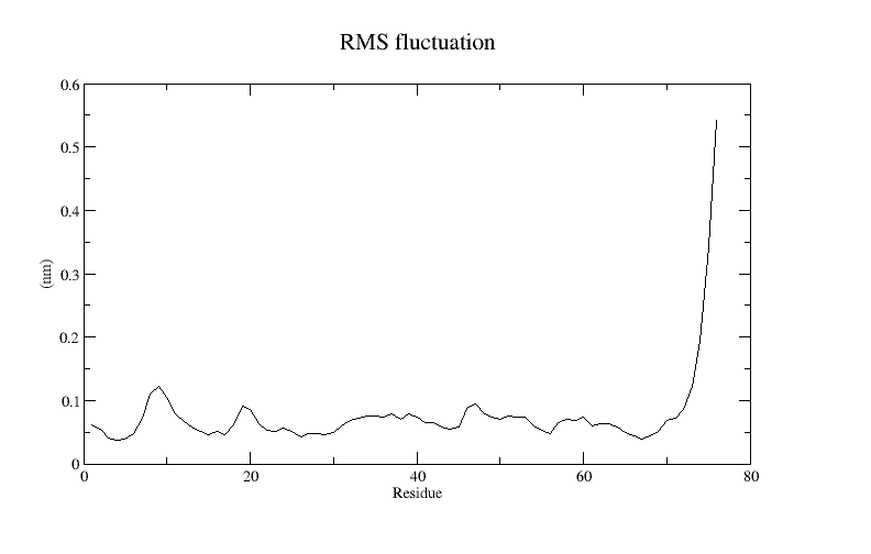
An alternative metric is to compute the root mean square fluctuatoins (RMSF). The RMSF captures, for each atom, the fluctuation about its average position. This gives insight into the flexibility of regions of the peptide. The RMSF (and the average structure) are calculated with the rmsf command. We are most interested in the fluctuations on a per residue basis, which is controlled by the flag -res.

$ gmx rmsf -s frame1.pdb -f md_trajectory_noPBC.xtc -o rmsf-per-residue.xvg -ox average.pdb -res

Have a look at the graph of the RMSF with xmgrace and identify the flexible and rigid regions of the protein.

xmgrace rmsf-per-residue.xvg

A plot of the RMSF for ubiquitin is shown below:

A side product of the RMSF calculation is the average protein structure over the course of the simulation. Note that the average protein structure is not necessarily a physically relevant structure if there are large conformational changes during the simulation. To get a better measure of the convergence of the simulation to equilibrium, we compute the RMSD again, but this time using the average structure as the reference structure.

$ gmx rms -s average.pdb -f md_trajectory_noPBC.xtc -o rmsd-vs-average.xvg

Again select 4 for the Backbone atoms for both the alignment and RMSD calculation.

Plot the generated rmsd-vs-average.xvg using the Xmgrace plotting tool

xmgrace rmsd-vs-average.xvg

A plot of the RMSD is shown below:

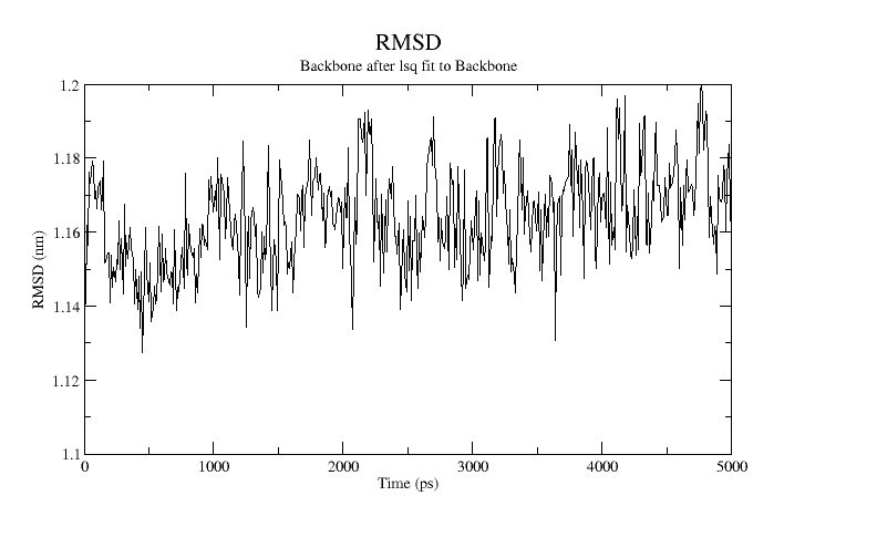
At equilibrium about a single stable configuration, the RMSD value should be level and fluctuate about the mean.

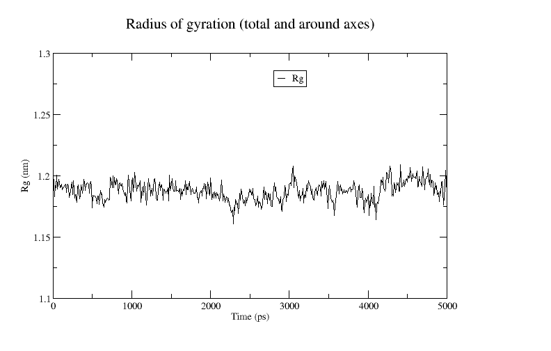
Radius of gyration

The module gyrate allows you to check the radius of gyration of the system. If the protein is unfolding or adopting “open” configurations, the radius of gyration will increase.

gmx gyrate -s frame1.pdb -f md_trajectory_noPBC.xtc -o gyrate.xvg

Plot the generated gyrate.xvg using the Xmgrace plotting tool

xmgrace gyrate.xvg

A plot of the radius of gyration is shown below:

Principal mode analysis of an MD trajectory

A very common method is to extract the “principal” or “essential” motions that have the largest amplitudes and involve the largest parts of the structure. Principal component analysis (PCA) of the trajectory, which is sometimes also referred to as ‘essential dynamics’ (ED), aims at identifying large scale collective motions of atoms and thus reveal the structures underlying the atomic fluctuations. The fluctuations of particles are correlated due to coupled interactions between particles. The degree of correlation will vary and notably particles which are directly connected through bonds or lie in the vicinity of each other will move in a concerted manner. The correlations between the motions of the particles give rise to collective motions in the system that is often directly related to its function or (bio)physical properties. The study of the structure of the atomic fluctuations can give valuable insight in the behavior of a macromolecule.

In principal component analysis the original data is transformed into new set of variables which are linear combinations of the original ones. The first step in PCA is the construction of the covariance matrix, which captures the degree of collinearity of atomic motions for each pair of atoms. This matrix is subsequently diagonalized, yielding a matrix of eigenvectors and a diagonal matrix of eigenvalues. Each of the eigenvectors describes a collective motion of particles, where the components of the vector indicate how much the corresponding atom participates in the motion. The associated eigenvalue is a measure of the total motility associated with an eigenvector. Usually most of the motion in the system (>90%) is described by less than 10 eigenvectors or principal components. Since the covariance analysis produces a lot of files, the analysis is best performed in a subdirectory below the directory of the MD run:

mkdir COVAR

cd COVAR

The program covar will construct the covariance matrix and perform the diagonalization. Issue the following command:

gmx covar -s ../frame1.pdb -f ../md_trajectory_noPBC.xtc -o eigenvalues.xvg -v eigenvectors.trr -xpma covar.xpm

Choose ‘Backbone’ for the analysis. First, have a look at the eigenvalues:

xmgrace eigenvalues.xvg

An example plot is shown here:

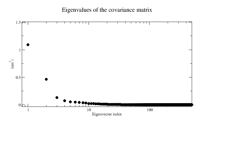
In the above example, we see that most of the eigenvalues are close to zero and that most of the motion can be described by only the first two eigenvectors. As we shall see, this motion correspond to the C-terminus tail fluctuations as seen in the large RMSF values above.

To see what the collective motions are that correspond to the eigenvectors we use the tool anaeig. Here we will look at just the first eigenvector corresponding to the largest eigenvalue. Issue the following command:

gmx anaeig -s ../frame1.pdb -f ../md_trajectory_noPBC.xtc -v eigenvectors.trr -eig eigenvalues.xvg -proj proj-ev1.xvg -extr ev1.pdb -rmsf rmsf-ev1.xvg -filt trajfilt1.pdb -first 1 -last 1

Choose again ‘Backbone’ for the analysis. The eigenvectors correspond to directions of motion. The option -extr extracts the extreme structures along the selected eigenvectors from the trajectory. The -filt option filters the trajectory to show only the motion along the eigenvectors -first to -last.

Loading the structure file ev1.pdb into PyMOL. The python script modevectors.py will allow us to plot the vectors and the movement along the trajectory. Within PyMOL, execute the command File -> Run Script… -> modevectors.py and then type in the consol

PyMOL> modevectors ev1, ev1, 1, 2, factor=1, headrgb=(1,0,0), tailrgb=(1,0,0), cutoff=0.5, outname=ev11

An example visualization of the first principal components is shown below.

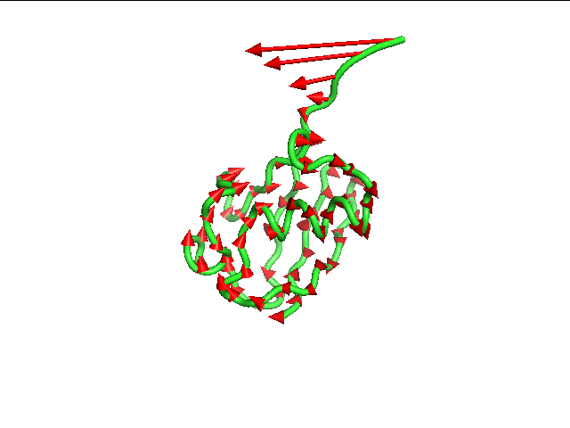
As we can see, this “principal” motion corresponds to the fluctuations of the C-terminus tail. In ubiquitination, the ubiquitin molecule covalently binds through its C-terminal carboxylate group to a particular lysine, cysteine, serine, threonine or N-terminus of the target protein. We see that the dynamics of the C-terminus is thus related to the biological function.