Basics of a GROMACS simulation

Add new Edit Delete History Source Add new post
Prose.io: Add new Edit Add new post

3 July 2019

Basics of a GROMACS simulation

About this tutorial

GROMACS is an open source program to run molecular dynamics (MD) simulations. This page contains some basic commands to set up and run a MD simulation. It is important that you understand what each command is doing and that you document for yourself all the simulation parameters that were chosen and details about how the system was built. To perform the simulation you will need some force field parameter files. These can be downloaded here.

Convert pdb structure file to GROMACS topology and structure file.

First we must download a protein structure file (pdb text file) from the RCSB website. In this tutorial will we use the protein ubiquitin. The RCSB pdb code for ubiquitin is 1UBQ.pdb and can be found here. Download the file in PDB format. You can visualize the structure using a viewing program such as VMD, Chimera, or PyMOL.

We first need to convert this pdb file to a format that Gromacs uses. The Gromacs command pdb2gmx will generate a Gromacs topology file (.top), a position restraint file (posre.itp), and a Gromacs structure file (.gro). Generating a topology file can sometimes be tricky if there are missing atoms, non-standard amino acids, or small molecules in the pdb file. A basic usage of pdb2gmx is

$ gmx pdb2gmx -f 1ubq.pdb -o 1ubq.gro -p 1ubq.top -ignh

where -f signals the input pdb file, here called 1ubq.pdb and -o is the output structure file and -p is the output topology file. The flag -ignh means to ignore H atoms in the PDB file. The -ignh flag is useful to deal with non-conventional naming of H atoms in pdb files; however, if you need to persevere the exact position of the H coordinates in the structure file, then you should not use the -ignh flag.

Typing the above command will prompt you to select a force field. Select the force field by typing the appropriate number and hitting the Enter/Return key. You will also be prompted to select a water model. For this tutorial select the AMBER99SB-ILDN force fields from Lindorff-Larsen et al., Proteins 78, 1950-58, 2010, and when prompted, select the TIP3P water model. You should now have generated a structure file 1ubq.gro, a topology file 1ubq.top, and a position restraint file posre.itp.

The topology file 1ubq.top contains all the information necessary to define the molecule within a simulation. This information includes nonbonded parameters (atom types and charges) as well as bonded parameters (bonds, angles, and dihedrals).

Defining a simulations box and adding solvent

Next, we define and create a simulation box of specified dimensions using the editconf command

$ gxm editconf -f 1ubq.gro -o 1ubq_newbox.gro -c -d 1.0 -bt cubic

The -f flag signals the input Gromacs structure file which we created above. The -o signals the new output structure file which contains the box definition. The -c flag centers the protein in the box, and the -d specifies a minimum distance from the protein to the edge of the box (in nm). Specifying a solute-box distance of 1.0 nm means that there are at least 2.0 nm between any two periodic images of a protein. This distance will be sufficient for just about any cutoff scheme commonly used in simulations. The -bt cubic flag indicates to use a cubic box shape. Now that we have generated a simulation box, which we must fill with water. We add solvent by typing

$ gmx solvate –cp 1ubq_newbox.gro –cs spc216.gro –o 1ubq_solv.gro –p 1ubq.top

The input structure file signaled by -cp 1ubq_newbox.gro is the structure file that was generated by the previous command. The -cs flag is the solvent configuration structure file that comes standard with a Gromacs installation. We are using spc216.gro, which is a generic equilibrated 3-point solvent model. You can use spc216.gro as the solvent configuration for SPC, SPC/E, or TIP3P water, since they are all three-point water models. The -o flag indicates a new output structure file that contains both the protein and the solvent. The -p flag is our topology file generated above, which will be modified to include the solvent force fields as well.

Adding ions

Usually, we will want to add small molecule ions (NaCl) in order to neutralize the system (if the protein has a nonzero net charge) and to perform the simulation at physiological or experimental salt conditions. The Gromacs command genion will randomly replace water molecules with ions. In order to run genion we need to generate a compiled Gromacs input file (.tpr) file called a run input file. A .tpr file contains information from both the structure file (.gro) and topology file (.tpr) and is generated using the grompp (Gromacs pre-processor) command, which will also be used later when we run our first simulation.

To produce a .tpr file, we need an additional input file with extension .mdp (molecular dynamics parameter file) that contains specified parameters for running a simulation. For this tutorial, you can use the ions.mdp file. We then generate the .tpr file as follows:

gmx grompp -f ions.mdp -c 1ubq_solv.gro -p 1ubq.top -o ions.tpr

where -o specifies the output .tpr file which we have called ions.tpr. We have now generated a compiled file called ions.tpr. Now we can add small ions with the command

gmx genion -s ions.tpr -o 1ubq_solv_ions.gro -p 1ubq.top -conc 0.15 -neutral

where the -conc signals to make the final ion concentration 0.15 M (physiological salt concentration) and -neutral signals to neutralize the system so that the net charge in the system is zero. Gromacs will randomly replace certain molecules with small ions to reach our specified concentration and charge balance. When prompted select group 13 for SOL, which is the solvent group. This will tell Gromacs to replace some of the solvent molecules with small ions. We now have a simulation box containing our protein, water, and salt. To run an MD simulation we need the generated Gromacs structure file (1ubq_solv_ions.gro) and the Gromacs topology file (1ubq.top).

Energy Minimization

Before we can run a MD simulation, we need to relax the system to remove steric clashes or unphysical geometries. To run an energy minimization we need another .mdp file that contains the parameters for the energy minimization. You can use the em.mdp file. Again we use the grompp command to compile a Gromacs .tpr file.

gmx grompp -f em.mdp -c 1ubq_solv_ions.gro -p 1ubq.top -o em.tpr

where -o signals the output em.tpr file. Now to run the energy minimization we use the Gromacs mdrun command

gmx mdrun -v -s em.tpr -o em.trr -x em.xtc -cpo em.cpt -c em.gro -e em.edr -g em.log

Here the -o signals the output full precision trajectory, the -x a compressed trajectory, the -cpo outputs a checkpoint file, the -c the output structure file, the -e signals the output energy file, and -g the output log file.

An alternative, abbreviated command you can use instead is to use the -deffnm flag to signal a default file name for all output files:

gmx mdrun -v -s em.tpr -deffnm em

The -v flag means “verbose” and means that Gromacs will print to the screen the minimization process each step. The -deffnm flag signals to make all output files the same name as the input file, here “em”. The output files will be em.log (ASCII-text log file), em.edr (binary energy file), em.trr (binary full-precision trajectory), and em.gro (the final energy minimized structure). It is a good idea to check how the total potential energy changes during the minimization. We can used the generated em.edr file for this analysis.

gmx energy -f em.edr -o potential.xvg

At the prompt, select “10” for the potential energy, and then hit “0” to terminate the input. Plot the generated potential.xvg using the Xmgrace plotting tool and see that the potential energy is converging to a minimum.

xmgrace potential.xvg

A plot of the potential energy is shown below:

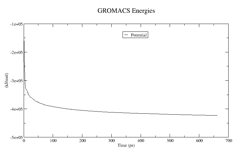
To verify the energy minimization was successful, the potential energy in (kJ/mol) should be negative, and (for a simple protein in water) on the order of –10⁵ to –10⁶, depending on the system size and number of water molecules.

Equilibration Run 1

Energy minimization from above optimizes the local geometry and solvent orientation. Before we can run a long MD trajectory, we still need to equilibrate the solvent molecules and ions around the protein at the temperature we wish to simulate. For the first phase of equilibration we will use an NVT ensemble (constant number of particles, volume and temperature). We will perform a short (100 ps) simulation with the protein positions restrained. Position restraints thus allow us to equilibrate the solvent around the protein, without causing significant structural changes in the protein. The restraint parameters are contained in the posre.itp file. Again we use a .mdp file containing the parameters for the simulation. These parameters are specified in the file nvt.mdp file.

We use the grompp command as before:

and mdrun just as we did at the energy minimization (EM) step

gmx grompp -f nvt.mdp -c em.gro -p 1ubq.top -o nvt.tpr -r em.gro

where em.gro is the energy-minimized structure from above.

Take note of a few parameters in the nvt.mdp file by opening this file in a text editor of your choice. A few important lines to note are:

define = -DPOSRES; This sets position restraint on the protein
gen_vel = yes; Initiates velocity generation. Using different random seeds (gen_seed) gives different initial velocities, and thus multiple (different) simulations can be conducted from the same starting structure.
tcoupl = V-rescale; The velocity rescaling thermostat is an improvement upon the Berendsen weak coupling method, which did not reproduce a correct kinetic ensemble.
pcoupl = no: Pressure coupling is not applied.

Finally we can run the molecular dynamics as follows

gmx mdrun -v -s nvt.tpr -deffnm nvt

When the equilibration is finished you can analyze the temperature progression

gmx energy -f nvt.edr -o temperature.xvg

Type “16 0” at the prompt to select the temperature of the system and exit. You can view the temperature progression using xmgrace

xmgrace temperature.xvg

A plot of the temperature is shown below:

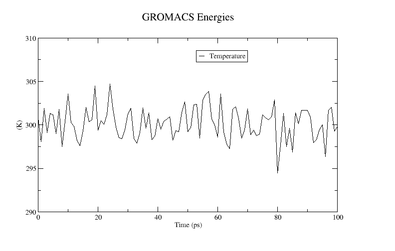
Here we can see that over the course of the 1 ps equilibration run, the temperature is fluctuating around 300 K as expected.

Additional Equilibration Runs

The previous step, NVT equilibration, stabilized the temperature of the system. If we want to perform the simulation in the NPT ensemble at a particular density, we also need to perform an equilibration in the NPT ensemble at a specified temperature and pressure to allow the system density to reach its equilibrated value. This can be done using the mdp file npt.mdp

Again we use the grompp command:

gmx grompp -f npt.mdp -c nvt.gro -p 1ubq.top -o npt.tpr -r nvt.gro -t nvt.cpt

where nvt.gro is the final structure from the previous nvt equilibration, and the -t flag signals to use the velocities from the checkpoint file from our previous nvt equilibration (continuation run). Note here we no longer include the position restraint on the protein. Additionally, in the npt.mdp file we have added the Parrinello-Rahman barostat

pcoupl      = Parrinello-Rahman   ; Pressure coupling is applied.
pcoupltype  = isotropic           ; uniform scaling of box vectors
tau_p = 2.0                       ; time constant, in ps
ref_p = 1.0                       ; reference pressure, in bar
compressibility = 4.5e-5          ; isothermal compressibility of water, bar^-1

Again we run the molecular dynamics as follows:

gmx mdrun -v -s npt.tpr -deffnm npt

When the run is finished you can analyze the pressure fluctuations

gmx energy -f npt.edr -o pressure.xvg

Type “17 0” at the prompt to select the pressure of the system and exit. View the pressure progression using xmgrace

xmgrace pressure.xvg

A plot of the pressure is shown below:

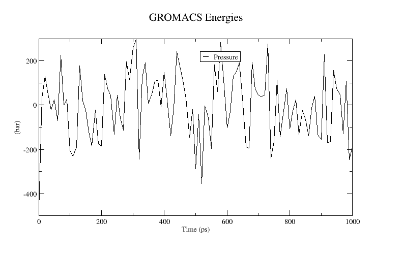
The instantaneous pressure value fluctuates widely over the course of the equilibration run, but this behavior is not unexpected. (Why do you think the instantaneous pressure fluctuates so much?) Over the course of the equilibration, the average value of the pressure is around 1 bar.

Often you will perform several equilibration steps to reach the desired target ensemble. Some common equilibration work-flows are show below. This figure taken from LivingJ.Comp.Mol.Sci.2019,1(1),5957

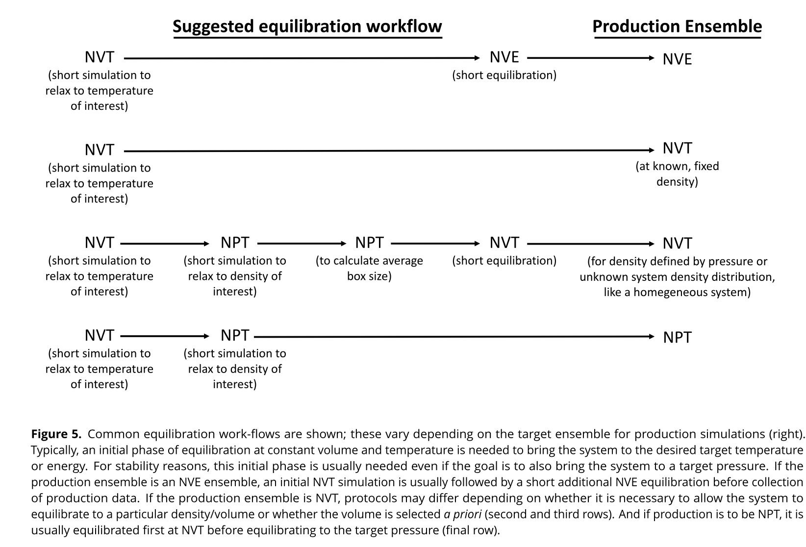
Note: the NPT equilibration here is short for the purpose of this tutorial. In practice, you should run a longer equilibration in the NPT ensemble and make sure the system is properly equilibrated by checking the RMSD

Production Run

Once the system has been equilibrated we can run a longer production run. Here we will perform the simulation in the NVT ensemble using the following mdp file production_nvt.mdp

in the production_nvt.mdp file we have extended the simulation time to 5 ns:

nsteps		= 2500000	; 2 * 2500000 = 50000 ps (5 ns)
dt		    = 0.002		; 2 fs

This is a short production run for this tutorial. For an actual production run, you would need to run the simulation for much longer.

Again, we use the grompp command:

gmx grompp -f production_nvt.mdp -c npt.gro -p 1ubq.top -o production_nvt.tpr -r npt.gro -t npt.cpt

where npt.gro is the final structure from the above npt equilibration and npt.cpt is the checkpoint file from the previous npt equilibration. And we run the production molecular dynamics as follows:

gmx mdrun -v -s production_nvt.tpr -deffnm production_nvt

This may take some time if running on a personal PC. Once it is finished you can check out the Analyzing a MD trajectory tutorial.

To run the job in the background in Linux, use the nohup command:

nohup gmx mdrun -v -s production_nvt.tpr -deffnm production_nvt >& nohup.log &

This will run the calculation in the background. Don’t forget to check the nohup.log file for any errors. Monitor the simulation progress using:

tail -f nohup.log

Extending the simulation time

Often we need to extend a simulation to add more time to the trajectory. For example, let’s say you have run a simulation for 100 ns and now want to extend the run to 200 ns. This can be done using the convert-tpr command. For example, if you want to extend the production_nvt.tpr file by 100 ns (100,000 ps), you can create a new tpr file using:

gmx convert-tpr -s production_nvt.tpr -o production_nvt_run2.tpr -extend 100000

Here the -extend signals how long to extend the simulation (in ps). Then, you can run the extended simulation using the checkpoint file:

gmx mdrun -v -s production_nvt_run2.tpr -cpi production_nvt.cpt -deffnm production_nvt_run2 -noappend

Note the -cpi signals to continue from the most recent checkpoint file from our previous simulation. The -noappend signals to not append to the previous outputs. In this case, you will get new output files with the prefix production_nvt_run2. Instead, if you want to append to the previous output files to generate one long continuous run, you can use:

gmx mdrun -s production_nvt_run2.tpr -cpi production_nvt.cpt -deffnm production_nvt

This will append the outputs to the previous production_nvt output files. Note that if you used the -deffnm in your original run, and you want appending, then your continuations must also use -deffnm. Appending will not work if any output files have been modified or removed after the mdrun wrote them.