Simulation of Liquid Argon

Add new Edit Delete History Source Add new post
Prose.io: Add new Edit Add new post

16 June 2022

Simulation of Liquid Argon

About this tutorial

In this tutorial you will learn how to perform a molecular dynamics (MD) of liquid argon using the GROMACS MD package. The goal will be to reproduce some of the results from the pioneering paper A. Rahman, “Correlations in the Motion of Atoms in Liquid Argon”, Phys. Rev. Lett. 136, A405, 1964.

Files to complete this tutorial can accessed here:
tutorial files

Introductory video about MD simulations to accompany this tutorial:
Video: Molecular Simulation
Video: Practical Exercise

MD simulation of argon

GROMACS is an open source MD simulation package. On the GROMACS homepage you can find more information about the software and documentation. To run a simulation, we need three input files:

a structure file, containing the atomic coordinates of the system to be simulated
a molecular topology file, containing the force field parameters, a description of the bonds, angles, etc …, of the system
a simulation parameter file, containing information about the type of simulation, number of steps, temperature, etc …

For the argon molecule, the atomic nuclei are treated as point particles and there are no bonds or angles. The starting structure was generated by placing point particles on a fcc lattice. To reproduce the results from A. Rahman’s 1964 paper, the system contains 864 argon atoms with a system density of 1.374 g/cm\(^3\)

Structure File

In this case, we will use a structure file in pdb format: Ar_864.pdb. Looking at the file we see that each atom has a number, an atom name Ar and a x,y,z position. You can read more about the pdb file format here

HEADER    simple PDB file with 864 atoms
CRYST1   34.681   34.681   34.681  90.00  90.00  90.00 P 1           1
ATOM      1 Ar   Ar  A   1       0.000   0.000   0.000  1.00  0.00
ATOM      2 Ar   Ar  A   2       2.890   2.890   0.000  1.00  0.00
ATOM      3 Ar   Ar  A   3       2.890   0.000   2.890  1.00  0.00
ATOM      4 Ar   Ar  A   4       0.000   2.890   2.890  1.00  0.00
...

To visualize the pdb format you can use VMD. In the terminal type:

vmd Ar_864.pdb

Now in the dropdown menu from the VMD Main window select Graphics –> Representations. In the Graphical Representations window select Drawing Method –> VDW (for van der Waals radius). You should see something that looks like:

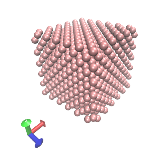
Notice that the argon atoms are arranged on a lattice to start.

Topology File

Now let’s have a look at the topology file argon.top. The atomtypes section contains information about the force field parameters for each atom type. Here we have one atom type AR for the argon atoms:

[ atomtypes ]
AR  39.948    0.0   A     0.006165     9.523537e-06

The first column defines the atom type parameters for the Argon atom. The second column is the mass in a.m.u. The third column is the charge. The last two columns are the parameters for the non-bonded interaction. You can find more information about these parameters here

MD Parameter File

The instructions to run the MD simulation are contained in the MD parameter file md_run.mdp. Have a look at this file. The beginning section defines the MD simulation run parameters. Here we use the leap-frog integrator with a time step of 0.002 ps for 50000 steps.

;Run parameters
integrator	= md		; leap-frog integrator
nsteps		= 50000		; 2 * 50000 = 100 ps
dt		= 0.002		; 2 fs

The next section controls how often to print to the output files that will be generated during the simulation. The remain sections specify more details about the simulation. The temperature is controlled with the following section:

; Temperature coupling is on
tcoupl		= v-rescale             ; modified Berendsen thermostat
tc-grps         = System
tau-t		= 0.1	        ; time constant, in ps
ref-t		= 94.4	        ; reference temperature, one for each group, in K

In the above we set the reference temperature to 94.4 K. The last section specifies that GROMACS should generate initial velocities of particles by randomly drawing from a Maxwell-Boltzmann distribution at 94.4 K.

; Velocity generation
gen_vel		= yes		; Velocity generation is on
gen_temp                 = 94.4 ; generate initial velocities at this temperature
gen_seed                 = -1

Generate GROMACS binary run input file and run the MD simulation

Running an MD simulation in GROMACS requires two steps. First, we use the Gromacs preprocessor command grompp to prepare a binary run input file that GROMACS can read and execute. Second, we run the simulation using the mdrun command. First run the GROMACS preprocessor by typing the following in the terminal:

gmx grompp -f md_run1.mdp -c Ar_864.pdb -p argon.top -o md_run1.tpr

Here the -f flag indicates the input MD parameter file, the -c flag indicates the input structure file, the -p flag indicates the input topology file. The -o flag specifies the output file name which is the binary run input file. Now we are ready to run the simulation using the mdrun command:

gmx mdrun -v -s md_run1.tpr -o md_run1.trr -x md_run1.xtc -cpo md_run1.cpt -c md_run1.gro -e md_run1.edr -g md_run1.log

The -s flag signals the input binary run input file. The rest of the flags indicate output files that will be produced as the simulation runs. The -o flag specifies the trajectory file, the -x flag specifies the output trajectory in compressed binary format, the -cpo flag is a checkpoint file, the -c flag is the output coordinates, the -e flag specifies the output energy file, and the -g flag indicates the output log file.

During this 100 ps simulation, the Argon atoms should melt from the lattice structure and become a liquid. The temperature should equilibrate to 94.4 K and the potential energy should reach a stable equilibrium. To check the temperature and energy, we can look at the instantaneous quantities in the md_run1.edr file. To check the temperature:

gmx energy -f md_run1.edr -o temperature.xvg -xvg none

Type “8 0” at the prompt to select the temperature and hit enter. The temperature.xvg file will have the time vs. temperature over the course of the simulation. You can plot this with any plotting tool. For example, in xmgrace:

xmgrace temperature.xvg

See if you can repeat this procedure to plot the potential energy. Does the potential energy reach a stable equilibrium?

Extending the Simulation

The first run was to melt the Argon atoms from the lattice and generate an equilibrated liquid at 94.4 K. Now we can run a longer simulation that we can use to compute properties of the liquid. Have a look at the MD parameter file: Ar_nvt.mdp. This file should look very similar to the previous MD parameter file with a few exceptions. First, we specify that this will be a continuation from a previous simulation. Second, we are no longer generating velocities since we are continuing from our previous simulation.

Now we run the GROMACS preprocessor to generate a new binary run input file for the longer simulation:

gmx grompp -f Ar_nvt.mdp -c md_run1.gro -t md_run1.cpt -p argon.top -o Ar_nvt.tpr

Notice here the input coordinate file is the md_run1.gro file that we generated in our previous simulation. This is the final coordinates from our equilibration simulation. Also, we have added the -t flag to indicate to restart the simulation from the previous checkpoint file. Now we run the simulation as before with:

gmx mdrun -v -s Ar_nvt.tpr -o Ar_nvt.trr -x Ar_nvt.xtc -cpo Ar_nvt.cpt -c Ar_nvt.gro -e Ar_nvt.edr -g Ar_nvt.log

This will generate a 1 ns (1000 ps) trajectory.

Visualizing the simulation

If we want to visualize the trajectory we can use vmd. Type in the terminal:

vmd Ar_nvt.xtc Ar_nvt.gro

Again go to Graphics –> Representations and choose Drawing Method –> VDW. You can now play the trajectory. Tip: You can also display the simulation box with the tcl command (type at the VMD> prompt:)

pbc box

Analyzing the simulation

To compute the radial distribution function type:

gmx rdf -s Ar_nvt.tpr -f Ar_nvt.xtc -o rdf.xvg -xvg none

When prompted select Group 0 for the ‘ref’ and Group 0 for the ‘sel’ and then type Ctrl-D to run the calculation. This will produce the output radial distribution function as a data file that you can plot in your favorite plotting program. For example, in xmgrace:

xmgrace rdf.xvg

An example is shown here:

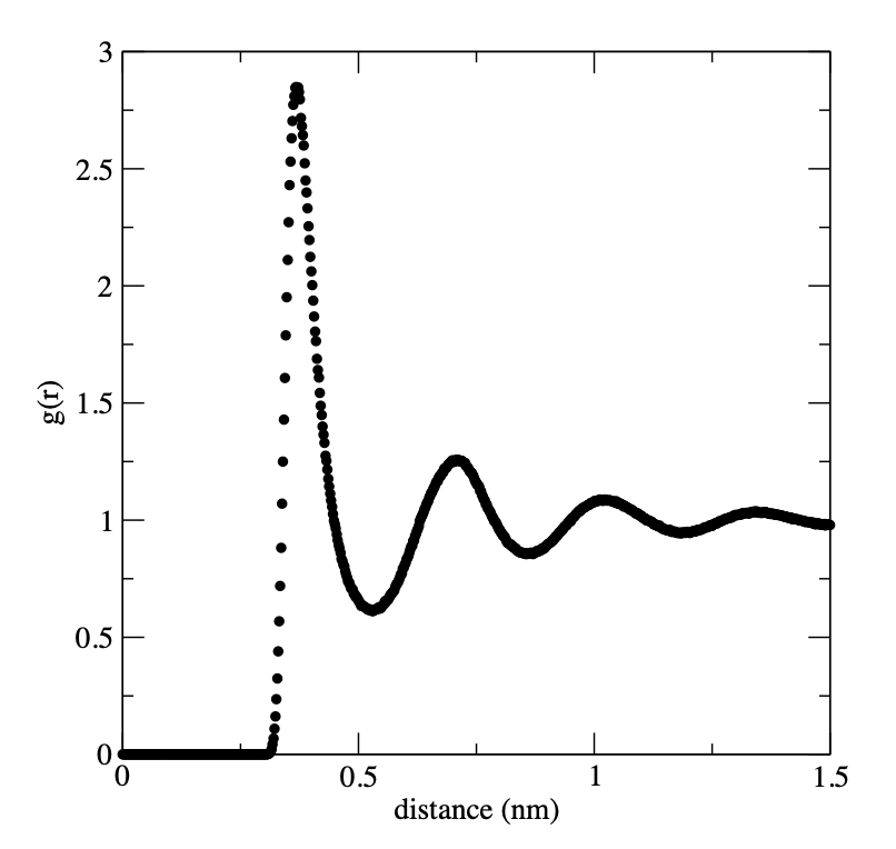
How does this compare with the results from Rahman’s 1964 paper?

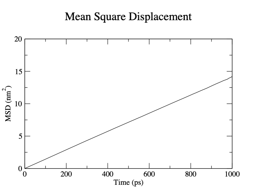
Another quantity of interest is the mean squared displacement of the atoms. This can be used to analyze the self diffusion of Ar atoms from the Einstein relation: \(\lim _{t \rightarrow \infty}\left\langle\left\|\mathbf{r}_{i}(t)-\mathbf{r}_{i}(0)\right\|^{2}\right\rangle=6 D t\)

To calculate the mean squared displacement:

gmx msd -s Ar_nvt.tpr -f Ar_nvt.xtc -o msd.xvg -xvg none

Select group 0 for System when prompted. Here we see that fitting the mean squred displacement from 100 to 900 ps gives:

D[   System ] 2.3474 (+/- 0.0467) 1e-5 cm^2/s

The value from Rahman’s 1964 paper is \(D=2.43\times 10^{-5}\) cm\(^2\)/s.

Extensions

A Lennard-Jones fluid can undergo a liquid to solid phase transition at low temperatures. The MD parameter file Ar_anneal.mdp will cool the system from 94.4 K to 10 K. To run this simulation starting from our previous simulation, type:

gmx grompp -f Ar_anneal.mdp -c Ar_nvt.gro -t Ar_nvt.cpt -p argon.top -o Ar_anneal.tpr

followed by

gmx mdrun -v -s Ar_anneal.tpr -o Ar_anneal.trr -x Ar_anneal.xtc -cpo Ar_anneal.cpt -c Ar_anneal.gro -e Ar_anneal.edr -g Ar_anneal.log

See if you can make a plot of the temperature as a function of the simulation time. Does the temperature behave as you expect?

When does the freezing begin?

Compute the radial distribution of the sold state by taking account of only the second half of the simulation.

gmx rdf -s Ar_anneal.tpr -f Ar_anneal.xtc -b 500 -o rdf_solid.xvg -xvg none

How does the radial distribution function compare to the liquid?

How do your results change for the smaller noble gas neon. (Hint: here is a set of simulation parameters for neon: neon.top)